Local equilibration
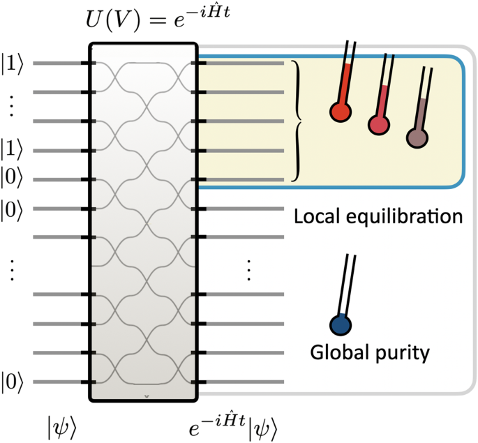
In any setting governed by closed-system Hamiltonian dynamics, equilibration can only happen locally for local observables since the global entropy must be preserved in time. In the setting considered, the global system is a multi-mode linear-optical system initially prepared in a highly non-Gaussian state ρ on m bosonic degrees of freedom, namely \(\left|\psi \right\rangle \left\langle \psi \right|\) with \(\left|\psi \right\rangle=\left|1,\ldots,\,1,\,0,\ldots,\,0\right\rangle\) of n = 3 single photons in m = 4 optical modes. The bosonic modes are associated with annihilation operators \({\hat{b}}_{1},\ldots,\,{\hat{b}}_{m}\). The subsequent integrated linear optical circuit is given by a unitary V ∈ U(m) that linearly transforms the bosonic modes. Any unitary from the group U(m) of m × m unitary matrices can be realized by a suitably designed linearly optical circuit. In state space, such linear optical circuits are reflected by ρ ↦ σ ≔ U(V)ρU(V)†, where U(V) is the physical implementation of the passive mode transformation V that linearly transforms a set of bosonic operators to a new set as \({({\hat{b}}_{1},\ldots,\,{\hat{b}}_{m})}^{T}\mapsto V{({\hat{b}}_{1},\ldots,\,{\hat{b}}_{m})}^{T}\). The representation of the mode transformation in Hilbert space V ↦ U(V) is commonly referred to as the metaplectic representation in technical terms. Finally, the output distribution is measured in the Fock basis using quasi-photon number resolving detectors, giving measurements of the form μ ↦ P(μ) with
$$P(\mu )=\langle {n}_{1},\ldots,\,{n}_{m}|U(V)\rho U{(V)}^{{{{\dagger}}} }|{n}_{1},\ldots,\,{n}_{m}\rangle,$$ (1)
where μ = (n 1 , …, n m ) is a given pattern of detection events.
For our purpose of showing local equilibration, we interpret the evolution \(U(V)={e}^{-i\hat{Ht}}\) as the evolution under a Hamiltonian \(\hat{H}\) for time t > 0, which distributes information. In the linear optical system at hand, we will implement two Hamiltonians, a quadratic bosonic translationally invariant ‘hopping’ Hamiltonian, resembling the non-interacting limit of a Bose-Hubbard Hamiltonian, and a Haar random transformation V ∈ U(m) corresponding to a Hamiltonian with random long-range interactions. In a fixed-size optical system, we can simulate the evolution at various times by tuning the strength of the evolution, interpreting t as scaling the strength rather than the duration of the interaction.
As the time t gets larger, increasingly longer-ranged entanglement builds up. This means that the expected moments of the local photon number \({\hat{n}}_{j}:={\hat{b}}_{j}^{{{{\dagger}}} }{\hat{b}}_{j}\) of each of the output modes labeled j = 1, …, m of the state σ will increasingly, in the depth of the circuit, equilibrate and lead to a distribution that resembles that of a (generalized) Gibbs ensemble. In other words, as seen in Fig. 1, one encounters local equilibration where the reduced quantum states of a subset of the modes, or individual modes, equilibrate and take thermal-like values. Equivalently, we can say that the state will locally thermalize in the sense that it results in the same expectation values for local observables as if the entire system had relaxed to a thermal equilibrium state.
Strictly speaking, here we observe a generalized thermalization in the following sense. The Gibbs or canonical state reflecting thermal equilibrium is given by \(\xi :={e}^{-\beta \hat{H}}/{{{{{{{\rm{tr}}}}}}}}({e}^{-\beta \hat{H}})\) for a suitable inverse temperature β > 0 that is set by the energy density. For non-interacting bosonic systems, local equilibration for subsystems consisting of several modes is instead expected to converge to a generalized Gibbs state. To be specific, here, the initial state is a product state (and hence has obviously short-ranged correlations)—albeit not being translationally invariant—and the bosonic quadratic Hamiltonian will, on the one hand, be translationally invariant before it undergoes a time evolution generated by \(U(V)={e}^{-i\hat{Ht}}\) (or the Haar-random V ∈ U(m)). The situation is particularly transparent where \(\hat{H}\) is a hopping Hamiltonian, which is translationally invariant. Defining the momentum space occupation numbers as
$${\hat{N}}_{k}:=\frac{1}{m}\mathop{\sum }\limits_{x,y=1}^{m}{e}^{2\pi ik(y-x)/m}{\hat{b}}_{x}^{{{{\dagger}}} }{\hat{b}}_{y}$$ (2)
one finds that the GGE is then given by the maximum-entropy state ω given by
$$\omega :=\,{{\mbox{argmax}}}\,\{S(\eta ):\,{{\mbox{tr}}}\,(\eta {\hat{N}}_{k})=\langle \psi|{\hat{N}}_{k}|\psi \rangle \,{{\mbox{for all}}}\,\,k\},$$ (3)
associated with an inverse temperature per momentum mode, where \(S(\eta )=-{{{{{{{\rm{tr}}}}}}}}(\eta \log \eta )\) is the von Neumann entropy. For an infinite system, convergence to such a state is guaranteed7,8,9,11, in the sense that the global pure state will remain pure, but again, all reduced states (and, for that matter, all expectation values of local observables) will for most times take the values of this GGE. For finite systems, it has been rigorously settled in what sense the state is locally approximated by such a GGE7,12,13,14,15 before recurrences set in. We discuss the specifics of this mechanism in more detail in Supplementary Note 2. For the Haar-random unitaries, we still find Gaussification in expectation, creating an interesting state of affairs, as here, the theoretical underpinning is less clear.
For subsystems consisting of a single bosonic mode only, canonical or Gibbs states, as well as GGEs, both give rise to identical photon number distributions reflecting Gaussian states: The state ‘Gaussifies’ in time. The situation at hand is particularly simple in the situation where the expectation value of the photon number is the same for each of the m output modes. Then for a Gaussian state, the probability of observing k photons reduces to
$$p(k)=\frac{\left({{n-k+m-2}\atop{n-k}}\right)}{\left({{n+m-1}\atop{n}}\right)}=\frac{{D}^{k}}{{(D+1)}^{k+1}}\left\{1+O\left(\frac{1}{m}\right)\right\},$$ (4)
where D ≔ n/m is the photon density per mode, which acts as an effective temperature.
Interestingly, GGEs are still not quite thermal or canonical Gibbs states, which would be maximum-entropy states given the expectation value of the energy, but a generalization of that state, due to the non-interacting nature of the Hamiltonian. For example, in full non-equilibrium dynamics under large-scale interacting Bose-Hubbard Hamiltonians (as can be probed with cold atoms in optical lattices21), one expects an apparent relaxation to a Gibbs state. In contrast, a GGE maximizes the von Neumann entropy under the constraint of the energy expectation and the momentum space occupation numbers, which are preserved under the non-interacting translationally invariant evolution \(t\,\mapsto \,{e}^{-i\hat{Ht}}\). Therefore, one can say that each of the momentum modes is then associated with its own temperature, as sketched in Fig. 1, and the system ‘thermalizes’ up to the constraints of the momentum space occupation numbers being preserved.
Such GGEs are also interesting from the perspective of quantum thermodynamics19,43,44. The presence of the additional conserved charges indeed alters the thermodynamic properties and comes in as a further constraint. It is also found that the minimum-work principle can break down in the presence of a large number of conserved quantities43. Resource theories for thermodynamic exchanges of non-commuting and hence non-Abelian observables are also strongly altered for GGEs compared to their thermal counterparts44.
Certification
In this section, we lay out the certification tools that we have developed to verify that the experiment has worked close to its anticipated functioning. Crucially, time evolution preserves the purity of a quantum system; the system only appears to be equilibrated when considering the local dynamics. Therefore, in the ideal case, it should be possible to undo the time evolution after applying U. This leads to the evolution U†U = I, meaning that a revival of the initial, non-Gaussian state is observed. In a noiseless experiment, this operation would function perfectly, and all entanglement will be formed between the photons as opposed to between the photons and the environment. This latter form of entanglement corresponds to decoherence and cannot be time-reversed by acting only on the photons. Therefore, the extent to which one observes a revival of the initial state serves as a measure of the degree of photon-photon entanglement versus the degree of decoherence.
We further formalize this idea in the form of a fidelity witness45,46 that certifies the fidelity \(F(\sigma,\,\left|{\psi }_{t}\right\rangle )=|\left\langle {\psi }_{t}\right|\sigma \left|{\psi }_{t}\right\rangle|\) between the experimentally prepared state σ and a pure target state described by a state vector \(\left|{\psi }_{t}\right\rangle :={e}^{-i\hat{Ht}}\left|\psi \right\rangle\). The procedure requires a well-calibrated, programmable measurement unitary and number-resolving (but not spectral-mode resolving) detectors. It consists of two settings for the measurement unitary: the inverse of the target unitary and the inverse followed by a Fourier transform U F . The constant number of measurement settings and polynomial classical computation resources required means the procedure is efficiently scalable to arbitrary system sizes. Here, we consider the specific case of witnessing against the specific target state of our experiment, leaving the generalization to Supplementary Note 1.
For the first measurement, we measure the state U†σU in the photon number basis. More specifically, we measure the fraction p 1 of detection events that correspond to our input state (i.e., exactly one photon in the first three input modes and no photon in the fourth mode). If our photodetectors would perfectly resolve the temporal and spectral degrees of freedom of the photons, this measurement in itself would be sufficient for certification45. However, in our system, the detectors only resolve the spatial mode. Neglecting this and naively carrying out the above procedure could result in certifying a large fidelity even with photons in distinct temporal modes, i.e., distinguishable states.
To rule this out, we employ an additional measurement setting as part of a two-step certification process: we implement U† followed by a Fourier transformation and count photons. From the first setting, we upper bound the probability p 1 of seeing one photon in each of the first three spatial modes and no photon in the fourth. From the second, we upper bound p 2 , the overlap probability of σ with the distinguishable sub-space. This is done by monitoring the fraction of observed interference patterns that would be forbidden for truly indistinguishable photons following a Fourier transform47,48,49.
In this way, we arrive at a fidelity bound of the form
$$F\ge {p}_{1}-\frac{9}{4}{p}_{2}-\delta (\epsilon )$$ (5)
where ϵ > 0 is the probability that the bound is correct, and δ is the corresponding statistical penalty, which arises from the observed photon counting statistics on p 1 and p 2 . This bound is derived from Chebyshev’s inequality and holds with very few assumptions on the underlying distribution (for a full derivation, see Supplementary Note 1).
If one is merely interested in establishing the presence of entanglement in the system, one can derive a simple entanglement witness \({{{{{{{\mathcal{W}}}}}}}}\) from the estimated fidelity. We use the following definition of an entanglement witness50
$${{{{{{{\mathcal{W}}}}}}}}:={\lambda }_{\max }^{2}{\mathbb{I}}-\left|{\psi }_{t}\right\rangle \left\langle {\psi }_{t}\right|$$ (6)
where \({\lambda }_{\max }^{2}\) is the maximal Schmidt coefficient in the decomposition of \(\left|{\psi }_{t}\right\rangle\) over a given partition, whose classical computation is not scalable but feasible in our case. It follows then that \(F\, > \,{\lambda }_{\max }^{2}\) is a witness of entanglement.
Integrated photonic platform
We use an integrated quantum photonics architecture as our experimental platform (see Fig. 2). Integrated quantum photonics constitutes a platform for non-universal quantum simulation based on bosonic interaction between indistinguishable photons27,51,52,53,54,55. In integrated quantum photonics, quantum states of light are fed into a large-scale tunable interferometer and measured by single-photon-sensitive detectors.
Our interferometer is realized in silicon nitride waveguides56,57, it has an overall size of n = 12 modes and an optical transmission of 2.2–2.7 dB, i.e., 54–60% depending on the input channel. Reconfigurability of the interferometer is achieved by a suitable arrangement of unit cells consisting of pairwise mode interactions realized as tuneable Mach-Zehnder interferometers58. Each unit cell of the interferometer is tuneable by the thermo-optic effect. For a full 12-mode transformation, the average amplitude fidelity \(F={n}^{-1}{{{{{{{\rm{Tr}}}}}}}}(|{U}_{{{{{{{{\rm{set}}}}}}}}}^{{{{\dagger}}} }||{U}_{{{{{{{{\rm{get}}}}}}}}}|)\) is F = 0.98, where U set and U get are the intended and achieved unitary transformations in the processor, respectively. The processor preserves the second-order coherence of the photons57.
We implement a quantum simulation of thermalization and a verification experiment in two separate sections of the interferometer. These two sections are indicated in blue and yellow, respectively, in Fig. 2; the area below the dotted line in Fig. 2 is not used. These two sections both form individual universal interferometers on the restricted space of four optical modes, allowing us to apply two arbitrary optical transformations U 1 and U 2 , in sequence.
We use the first section to simulate the time evolution of our input state. We select two families of Hamiltonians to simulate: A hopping Hamiltonian \({\hat{H}}_{{{{{{{{\rm{NN}}}}}}}}}=\gamma {\sum }_{k}{\hat{b}}_{k}^{{{{\dagger}}} }{\hat{b}}_{k+1}+{{{{{{{\rm{h.c.}}}}}}}}\) which consists of equal-strength nearest-neighbor interactions between all modes, which simulates the superfluid, non-interacting limit of the Bose-Hubbard model, and a set of 20 randomly chosen long-range Hamiltonians \({\hat{H}}_{{{{{{{{\rm{LR}}}}}}}}}={\sum }_{i,j}{\gamma }_{i,j}{\hat{b}}_{j}^{{{{\dagger}}} }{\hat{b}}_{i}+{{{{{{{\rm{h.}}}}}}}}\,{{{{{{{\rm{c.}}}}}}}}\), which we generate by applying the matrix logarithm to a set of Haar-random unitary matrices59.
The second section of the interferometer, indicated in Fig. 2 in yellow, is used for certification. When we wish to directly measure the quantum state generated by the first section, we set this area to the identity, leaving the state after U 1 untouched. However, we can also use this second section to make measurements in an arbitrary basis on the quantum state generated by U 1 , which allows us to certify the closeness of our produced quantum state to the ideal case.
Our photon source is a pair of periodically poled potassium titanyl phosphate (ppKTP) crystals operated in a Type-II degenerate configuration, converting light from 775 to 1550 nm60, with an output bandwidth of Δλ ≈ 20 nm. By using a single external herald detector and conditioning on the detection of three photons after the chip, we post-select on the state vector \(\left|\psi \right\rangle=\left|1,\,1,\,1,\,0\right\rangle\)52. By tuning the relative arrival times of our photons, we can continuously tune the degree of distinguishability between our photons. On-chip measurements via the Hong-Ou-Mandel (HOM) effect61 lower bound the wave function overlap between photons x = ∣〈ψ i ∣ψ j 〉∣, according to V = x2, where \(\left|{\psi }_{i}\right\rangle\) is the wave function of photon i, and V is the visibility of the HOM dip. We measure the visibility of 89% and 92% for photons of different sources and 94% for photons of the same source. Photon detection is achieved with a bank of 13 superconducting single-photon detectors62,63, which are read out with standard correlation electronics. For each of our four modes of interest, we multiplexed three detectors to achieve quasi-photon number resolution64, with the thirteenth detector used as the herald. By means of adjusting the time delay between the photons, we can adjust their degree of mutual distinguishability. We can switch between indistinguishable particles, which produce an overall entangled state (i.e., exhibiting both modal and particle entanglement), which will exhibit thermalization, and distinguishable particles, in which each photon traverses the experiment unaffected by the others, corresponding to a product state of the single-photon wave functions, which does not exhibit local thermalization.
Experimental results
Figure 3 shows the results of our quantum simulation of the hopping Hamiltonian and 20 random instances of longe-range Hamiltonians in sub-figures (a) and (b), respectively. The two sub-figures each have a tabular structure, where the columns indicate the different simulated time steps, with the simulation time indicated at the head of the column, and the rows indicate different measurement settings, i.e., either the experiment itself or the corresponding certification measurements. The data in these figures were acquired over 20 min for the photon number distribution, 320 min per certification measurement for the hopping Hamiltonian, and 220 min for each certification measurement of the long-range Hamiltonian, with four-photon events (three photos in the processor plus herald) occurring at a rate of 4 Hz.
Fig. 3: Quantum simulation of single- and multi-mode measurements. a Hopping Hamiltonian (superfluid): In panel I, the time evolution of photon-number probability distribution in spatial output mode 1 is plotted. The black points (squares) show the theoretical prediction for indistinguishable (distinguishable) particles, while colored points correspond to experimental data. Panels II–IV show the observed output distributions. These rows correspond to the output distributions of the hopping Hamiltonian (panel II), the first certification measurement U−1 (panel III), and the second certification measurement U F U−1 (panel IV). Theoretical predictions (Th) are represented by bars, and the experimental results (Exp) are represented by circles. The green-colored data corresponds with outcomes that benefit the certification protocol, whereas the red data is forbidden, i.e., ideally, should not occur. b Long-range Hamiltonian (Haar random): In panel I, the time evolution of photon-number probability distribution in spatial output mode 1 for 20 different random Hamiltonians is plotted. The black points (squares) show the theoretical prediction for indistinguishable (distinguishable) particles, while colored points correspond to experimental data. Panels II–IV show the observed output distributions for the first long-range Hamiltonian. These rows correspond to the output distributions of the first long-range Hamiltonian (panel II), the first certification measurement U−1 (panel III), and the second certification measurement U F U−1 (panel IV). Theoretical predictions (Th) are represented by bars, and the experimental results (Exp) are represented by circles. The green-colored data corresponds with outcomes that benefit the certification protocol, whereas the red data is forbidden, i.e., ideally, should not occur. Full size image
The first row of the two sub-figures displays the single-mode photon-number statistics k ↦ p(k) as generated after the application of U in the first section of the processor. The output statistics were measured for the first output mode. The experiment was carried out for both distinguishable (blue points) and indistinguishable (red points) photons. The gray bars show the expected distribution at full equilibration given by Eq. (4). For both Hamiltonians, initially, the input state is still clearly present, as indicated by the high probability of observing exactly one photon in the observed output mode. However, entanglement builds up as time evolves since the photons increasingly equilibrate. Consequently, for the indistinguishable photons, the initial input state evolves to a thermal-like state at t = 1. For both Hamiltonians, the distinguishable photons (whose output statistics correspond to those of classical particles) do not approach the canonical thermal state, demonstrating the intrinsic link between entanglement and thermalization.
For the hopping Hamiltonian, at later times (t = 2, t = 5), the finite size of our Hamiltonian gives rise to a recurrence, i.e., the state moves away from equilibrium again and evolves back towards the initial input state7,8. For the long-range Hamiltonian, in contrast, the long-range interactions mean that recurrences are pushed away to a later time not included in the simulation. These results suggest the presence of long-range order (as opposed to structured, nearest-neighbor interactions) tends to increase the time for which a system will continue to exhibit local relaxation. While this picture is intuitive, a rigorous understanding of these effects is an exciting open problem for theory and future experiments. The general agreement across a large range of randomly chosen Hamiltonians also represents strong experimental evidence for the ubiquity of these effects5,6.
The second row of the two sub-figures shows the full output-state distribution μ ↦ p(μ) after only the application of U, measured with indistinguishable photons. The bars in the background correspond to the expected distributions. For the long-range Hamiltonian, a single representative example of our 20 Hamiltonians is plotted. From this data, it can be clearly seen that at the point of thermalization, the photons are spread over many possible output configurations, whereas a recurrence manifests as a transition back to fewer possible output configurations.
The third and fourth rows show the output-state distributions after the first and second certification measurement, respectively. In these rows, the output configurations which contribute positively to the fidelity witness are indicated in green, and those which contribute negatively are indicated in red. The first certification measurement undoes the entanglement generated by U and ideally only results in state vectors of the form \(\left|{\psi }_{{{{{{{{\rm{out}}}}}}}}}\right\rangle=\left|1,\,1,\,1,\,0\right\rangle\). The second certification measurement also applies a three-mode Fourier to the generated states. Ideally, this results in only four allowed output configurations. These certification measurements show good agreement with the ideal allowed states, demonstrating a high degree of control over the experiment. For the second certification measurement, most of the deviations from the expected distribution can be attributed to the known photon indistinguishability. From the data presented in the third and fourth row, we extract the values of p 1 and p 2 , respectively, which are used in the fidelity witness as laid out in Eq. (5).
Figure 4a, b shows the certified fidelities for both the hopping Hamiltonian and the first random long-range Hamiltonian, respectively. The three horizontal ticks on each data point correspond to confidence values of ϵ = 0.7, ϵ = 0.8, and ϵ = 0.9. The line shows the entanglement witness, corresponding to a bi-partition between mode 1 and the remaining modes. The relatively constant fidelity to the target global state contrasts against the conversion of the local, single-mode statistics to thermal statistics, as seen in Fig. 3.
Fig. 4: Global state fidelity certification. a Certification of entanglement in the hopping Hamiltonian (superfluid): The lower bound certification fidelity estimations for the hopping Hamiltonian are plotted against a theoretical entanglement witness. b Certification of entanglement in the first long-range Hamiltonian (Haar random): The lower bound certification fidelity estimations for the first long-range Hamiltonian are plotted against a theoretical entanglement witness. In both plots, the top, middle, and bottom points at each time step correspond to confidence values of ϵ = 0.7, ϵ = 0.8, and ϵ = 0.9, respectively. The background color saturation qualitatively shows the total entanglement generated at that time step, which is proportional to the value of the entanglement witness. A higher saturation indicates a stronger presence of multi-photon entanglement. Full size image
Figure 4 a) shows that entanglement is certified for t = 1 in the hopping Hamiltonian system. The observed fidelity F = 0.359 is above the threshold of the entanglement witness. Similarly, Fig. 4b) shows an unambiguous certification for the first long-range Hamiltonian at t = 2. The fidelity F = 0.360 is well above the certification threshold. Both of these entanglement certifications hold with a confidence of at least 90%.