Moisture tracking in SSPs
We used UTrack, a Lagrangian atmospheric moisture tracking model, to track moisture forwards in time from evaporation to precipitation5,84. Being a three-dimensional Lagrangian tracking model that reconstructs moisture trajectories using evaporation and precipitation directly, UTrack is conceptually similar to some other Lagrangian methods85,86, but differs from other widely used tracking methods that are Eulerian87 or follow changes in specific humidity instead88. Using UTrack, we tracked the three-dimensional atmospheric trajectories of large numbers of individual ‘parcels’ of moisture and updated their positions every time step of 4 h based on evaporation, precipitation, humidity levels and three-dimensional wind speeds and directions. The respective forcing data were output of the medium-resolution Norwegian Earth System Model version 2 (NorESM2)89, which provides sufficiently detailed model output for UTrack and comprises all tier 1 scenarios in ScenarioMIP90 up until 2100: SSP1-2.6, SSP2-4.5, SSP3-7.0 and SSP5-8.5. Furthermore, it outperforms most CMIP6 models on reproducing historical observations of the hydrological cycle91,92. NorESM2 has a temporal resolution of 1 day and a spatial resolution of 1.25° × 0.9375°. We performed forward tracking from each of the 416 grid cells in the Amazon basin for each month and SSP. For each mm of evaporation at each grid cell during each time step of 4 h, we released 100 moisture parcels at random locations above the starting grid cell. Consistent with the ERA5-based UTrack model84, this time step is considerably smaller than the temporal resolution of the forcing data, to prevent skipping of grid cells by parcels during a time step. The wind speeds are calculated for eight pressure levels: 1,000 hPa, 850 hPa, 700 hPa, 500 hPa, 250 hPa, 100 hPa, 50 hPa and 10 hPa. To compensate for underestimated vertical mixing of moisture in the forcing data, each parcel is additionally assigned an occasional quasi-random repositioning along the atmospheric column. This is set such that on average once every 24 h, a parcel repositions itself vertically, where the probability of the new position is weighted by the specific humidity along the column5,84. The moisture content of the parcels is updated if precipitation occurs at that time step in the grid cell corresponding to the position of the parcel and the precipitation moisture is allocated to that grid cell. The tracking and updating continue until 99% of the original moisture in the parcel has been allocated to precipitation or after 30 days have passed since parcel release. It is important to note that, as opposed to ref. 5, we tracked evapotranspiration from each grid cell of the Amazon separately, and stored the results per grid cell, per month and per SSP. As we released 100 parcels per mm of evapotranspiration for each grid cell, this results overall in more than 1 billion parcel releases for this study. As such, although previous studies analysed moisture recycling for the Amazon in CMIP5 (ref. 93) and CMIP6 (refs. 5,94) models, we present grid cell-to-grid cell simulations, enabling us to construct the full moisture flow network. Finally, we validated the NorESM2 wind speed data for the Amazon and the Amazon precipitation recycling ratios using ERA5 reanalysis data and ERA5-forced UTrack runs. We show good correspondence between them and find no systematic bias that can explain our main transition risk results. We present these results in the Supplementary Information (Supplementary Note (Validation of moisture recycling based on EAR5 reanalysis data) and Supplementary Figs. 13–18).
Environmental data
We used MAP and evaporation values (to construct MCWD) from NorESM2 for the adaptation period from 1950 to 2014 (see the ‘Adaptation’ section) as well as for the four SSP scenarios that we used. For the three scenarios SSP2-4.5, SSP3-7.0 and SSP5-8.5, we evaluate the entire century using the now available moisture tracking data (2021–2099) while, for SSP1-2.6, we evaluate the decade 2090–2099 only. MAP and MCWD are computed as 10-year averages to cancel out the effects of single years that are particularly dry or wet. We use 10-year averages to capture long-term climatic shifts that drive system-wide vegetation changes, as supported by rainfall exclusion experiments showing that Amazon forests typically respond to sustained drought conditions over timescales of ten years1,47,65,95. While individual drought years can be impactful, especially for large trees, long-term stress is more relevant for assessing transition dynamics at the basin scale. Moreover, instead of calendar years, we account for dry and wet season conditions by using hydrological years. Hydrological years start in October of one year and run until September of the following year. MAP is computed from adding the corresponding monthly precipitation data in the respective hydrological year. For MCWD, we follow ref. 24 and compute the cumulative water deficit (CWD) from the according monthly precipitation and evaporation values using hydrological years:
$$\begin{array}{rcl} & & {\rm{M}}{\rm{C}}{\rm{W}}{\rm{D}}={\rm{a}}{\rm{b}}{\rm{s}}[\min ({{\rm{C}}{\rm{W}}{\rm{D}}}_{i},{{\rm{C}}{\rm{W}}{\rm{D}}}_{i+1},\ldots ,{{\rm{C}}{\rm{W}}{\rm{D}}}_{i+11})],\\ & & {\rm{w}}{\rm{i}}{\rm{t}}{\rm{h}}\,{{\rm{C}}{\rm{W}}{\rm{D}}}_{i-1}+{{\rm{P}}{\rm{r}}{\rm{e}}{\rm{c}}{\rm{i}}{\rm{p}}{\rm{i}}{\rm{t}}{\rm{a}}{\rm{t}}{\rm{i}}{\rm{o}}{\rm{n}}}_{i}-\,{{\rm{E}}{\rm{v}}{\rm{a}}{\rm{p}}{\rm{o}}{\rm{r}}{\rm{a}}{\rm{t}}{\rm{i}}{\rm{o}}{\rm{n}}}_{i}\\ & & {\rm{a}}{\rm{n}}{\rm{d}}\,\max ({{\rm{C}}{\rm{W}}{\rm{D}}}_{i})=0\end{array}.$$ (1)
Note that we use absolute values of MCWD in this study. While we use monthly precipitation values and evaporation values directly from NorESM2, the resulting global warming levels (from the SSP scenarios) are based on the wider spread of the CMIP6 database to not rely on a single Earth system model and its specific equilibrium climate sensitivity. Specifically, we use the median global temperature change as simulated in MAGICC7 (based on Fig. 4.40a of ref. 96).
Deforestation data
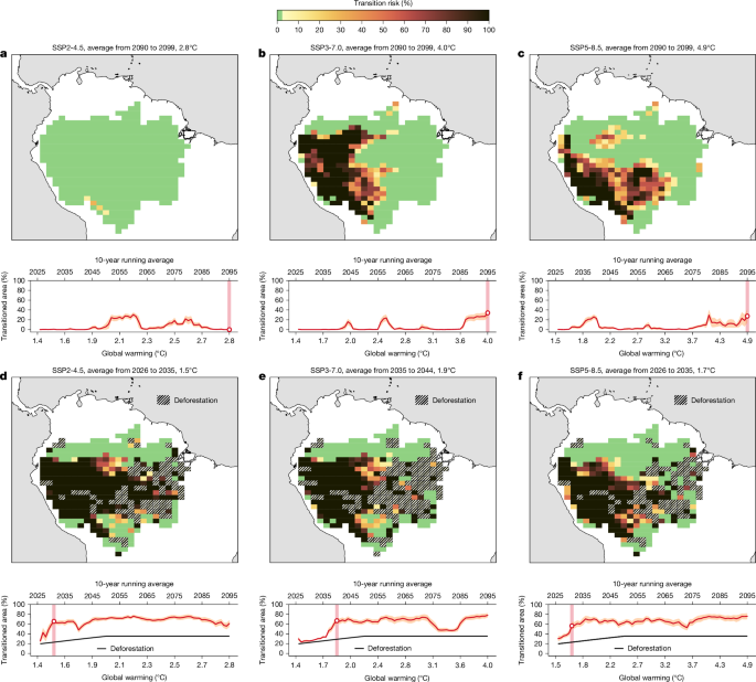
The deforestation data sets are taken from two different data sources. First, we use a severe deforestation data set that originates from ref. 70 and covers the Amazon basin from 2002 to 2050. This scenario assumes that the deforestation trends across the basin continue as well as additional deforestation occurring at locations of (planned) road pavements. At the same time, existing and proposed protected areas are ignored as reasons to limit or stop deforestation at these locations97. The projected deforestation rates were constructed by using historical images and their variations from 1997 to 2002 and then added to the effect of paving a set of major roads. We converted and regridded these data to the same grid as the environmental data, and kept deforestation levels from 2050 constant until the end of the century. From 2020 to 2050, the deforestation increased from ~0.55 million km2 to ~0.9 million km2 in this scenario (that is, from 18% to 35% of the Amazon basin being cleared), leading to an average yearly deforestation of ~18,000 km2 in this period. Despite the fact that the deforestation data are already a bit old, they uniquely project plausible Amazonian deforestation pathways until mid-century, explicitly linked to major infrastructure projects. Thus, the data enable a systematic assessment of critical deforestation thresholds relevant for analysing potential transitions. Second, we also include the deforestation scenarios following the respective SSP-based land use change scenarios (Supplementary Fig. 7). These are conservative scenarios with very limited deforestation after 2020 and none of these scenarios crosses the 25% level of basin-wide deforestation. Furthermore, most deforestation takes place in the west of the Amazon basin rather than in the east where vulnerabilities would be transported downwind.
Adaptation
Forests are not uniformly adapted to local climate conditions54,55,98. Various strategies exist both within and among forests to manage dry seasons and extreme droughts. We assume that local climate conditions have probably driven specific forest trait adaptations through processes such as environmental filtering, competitive exclusion and resilience. Specifically, we assume that forest ecosystems spread throughout the Amazon forest system are adapted to local adaptation values (here on a ~1° × 1° basis). This means that each grid cell is adapted to its past local environmental conditions. Our adaptation period ranges from 1950 to 2014 and includes the consistent historical simulation run, at which the four different SSP scenarios are branched off. Thus, the adaptation period is 1950–2014, while we evaluate the transition risk in the experimental period that ranges from 2021 to 2099 (averaged over a 10-year running average). With adaptation to past local conditions, we mean that the forest cells are adapted to their past MAP and MCWD values in the adaptation period, that is, to local precipitation and drought intensity values. Thus, they represent a local-scale tipping element with a threshold at MAP or MCWD values representing drier conditions than, on average, 1 s.d. away from those in the adaptation period. Locally, this means that critical thresholds can be vastly different; for example, drier regions in the Amazon forest are also capable of surviving drier conditions in the future. Overall, 1 s.d. is a conservative choice as losing 1 s.d. of moisture means on average losing around 25% of its MAP (Extended Data Fig. 4 and Supplementary Fig. 11), or becoming approximately 33% drier (that is, dry season intensity increase; Extended Data Fig. 4 and Supplementary Fig. 11). With this procedure, we are following and extending ref. 45, and follow the hypothesis that safety margins of forest ecosystems to droughts are similar regardless of the present (local) MAP58. However, we also find that our results are robust to the assumption that drier regions have lower safety margins than wetter regions as well as the other way round (see the ‘Robustness checks’ section for details). Lastly, although much of the forest may be adapted to local drought conditions, absolute thresholds are likely to exist for critical transitions in the Amazon forest system1,63 beyond which trees cannot survive. Thus, we ran a robustness analysis taking into account local adaptation as well as discrete thresholds in MAP and MCWD, in which the hard-wired thresholds follow the recent review on critical transitions in the Amazon forest1 with robust results in a qualitative and quantitative sense (see the ‘Robustness checks’ section for details).
Ensemble construction
As ecological adaptation varies stochastically across the Amazon forest system, they are drawn from a uniform distribution between 0.75 and 1.25 s.d. based on the values for MAP and MCWD of the local forest grid cell. These locally different adaptation values account for random variations in, for example, stomatal closure or heightened respiration. Ultimately, for each SSP scenario in each analysed decade, we draw ten different samples that are randomly drawn values for each cell from σ i ∈ [0.75; 1.25] for i = 1, 2, ..., N grid cells with 416 grid cells. As mentioned earlier, the precise value of adaptation is uncertain and may vary across different regions, influenced by several factors that are not explicitly modelled in this study such as the soil quality or competition of different species. To cover these uncertainties, we create a large ensemble and compute transition risks across the Amazon forest. Our ensemble size amounts to more than 1.25 million simulations (>3,000 simulations per grid cell), including all of our robustness checks.
Interacting dynamical systems approach
We extend the methodology developed in earlier literature45,68, where individual grid cells are modelled as interacting differential equations as follows:
$$\frac{{\rm{d}}{x}_{i}}{{\rm{d}}t}=-{x}_{i}^{3}+{x}_{i}+{C}_{{\rm{c}}{\rm{r}}{\rm{i}}{\rm{t}},i}({\rm{M}}{\rm{A}}{{\rm{P}}}_{i},{\rm{M}}{\rm{C}}{\rm{W}}{{\rm{D}}}_{i})+\mathop{\sum }\limits_{k=1,k
e i}^{{N}_{{\rm{g}}{\rm{r}}{\rm{i}}{\rm{d}}{\rm{c}}{\rm{e}}{\rm{l}}{\rm{l}}{\rm{s}}}}{R}_{ki}(\Delta {\rm{M}}{\rm{A}}{{\rm{P}}}_{ki},\Delta {\rm{M}}{\rm{C}}{\rm{W}}{{\rm{D}}}_{ki})\frac{{x}_{k}}{2}.$$ (2)
Here, each grid cell is modelled as a nonlinear dynamical system with two alternative stable equilibria, representing a forest state and an alternative state (Extended Data Fig. 2). A transition occurs when hydroclimatic forcing (changes in MAP or MCWD) or the loss of stabilizing moisture inputs causes the forest equilibrium to lose stability, after which internal feedbacks drive the system towards the alternative state. This nonlinear equation is a typical dynamical system equation that can exhibit tipping point behaviour, where C crit and the summation terms can be interpreted as a time-evolving bifurcation parameter. Their dynamics follow the normal form of a fold bifurcation, a standard representation of threshold-driven regime shifts in ecological and climate systems68,99,100,101. While such dynamics are consistent with hysteresis and limited reversibility, reversed forcing is not simulated in our experiment as SSP2-4.5, SSP3-7.0 and SSP5-8.5 are not overshoot scenarios. In equation (2), x i represents the state of the forest at grid cell i, where x i = −1 is forest and x i = +1 is the alternative state, which is an (open-canopy) degraded ecosystem state (for example, a savanna or dry degraded forest state). The tipping point (transition threshold) with respect to two critical parameters MAP and MCWD is located at
$$\begin{array}{c}{C}_{{\rm{c}}{\rm{r}}{\rm{i}}{\rm{t}},i}({\rm{M}}{\rm{A}}{{\rm{P}}}_{i},{\rm{M}}{\rm{C}}{\rm{W}}{{\rm{D}}}_{i})=\text{max}(C({\rm{M}}{\rm{A}}{{\rm{P}}}_{i}),C({\rm{M}}{\rm{C}}{\rm{W}}{{\rm{D}}}_{i}))\\ \,+\left(1-\frac{\text{max}(C({\rm{M}}{\rm{A}}{{\rm{P}}}_{i}),C({\rm{M}}{\rm{C}}{\rm{W}}{{\rm{D}}}_{i}))}{\sqrt{\frac{4}{27}}}\right)\\ \,\times \text{min}(C({\rm{M}}{\rm{A}}{{\rm{P}}}_{i}),C({\rm{M}}{\rm{C}}{\rm{W}}{{\rm{D}}}_{i}))\end{array}$$ (3)
with the components
$$\begin{array}{c}C({\rm{M}}{\rm{A}}{{\rm{P}}}_{i})=\sqrt{\frac{4}{27}}\times {\left(\frac{{\rm{M}}{\rm{A}}{{\rm{P}}}_{i}-{\mu }_{{\rm{M}}{\rm{A}}{\rm{P}},i}}{{\rm{M}}{\rm{A}}{{\rm{P}}}_{{\rm{c}}{\rm{r}}{\rm{i}}{\rm{t}},i}-{\mu }_{\mathrm{MAP},i}}\right)}^{-1}\\ C({\rm{M}}{\rm{C}}{\rm{W}}{{\rm{D}}}_{i})=\sqrt{\frac{4}{27}}\times \frac{{\rm{M}}{\rm{C}}{\rm{W}}{{\rm{D}}}_{i}-{\mu }_{{\rm{M}}{\rm{C}}{\rm{W}}{\rm{D}},i}}{{\rm{M}}{\rm{C}}{\rm{W}}{{\rm{D}}}_{{\rm{c}}{\rm{r}}{\rm{i}}{\rm{t}},i}-{\mu }_{{\rm{M}}{\rm{C}}{\rm{W}}{\rm{D}},i}}\end{array}.$$ (4)
μ MAP,i is the grid cell-specific long-term average from the adaptation period (1950–2014) and MAP crit,i is the tipping point with MAP crit,i = μ MAP,i − σ i × Δ MAP,i , where Δ MAP,i is the local adaptive capacity of the grid cell to its past environmental conditions, which is measured as the s.d. from 1950 to 2014. This means that a region that experienced larger environmental fluctuations in the past is also adapted (that is, resilient) to such environmental fluctuations in the future. This is the mechanism with which we implement local adaptive capacities of the biosphere dependent on local past environmental conditions. σ i ∈ [0.75; 1.25] is the uncertainty in the adaptive capacity, on which we construct our ensemble (see the ‘Ensemble construction’ section). While drier conditions are represented by larger MCWD values (see equation (1)), they are also represented by lower values of MAP. Thus, the exponent −1 is needed in equation (4). Lastly, the specific critical value of \(\sqrt{\frac{4}{27}}\) is derived from the normal form of equation (2), and more details can be found in literature99,102.
Moreover, the moisture recycling network is parameterized in the last term of equation (2), where \({R}_{ki}={R}_{ki}(\Delta {{\rm{M}}{\rm{A}}{\rm{P}}}_{ki},\Delta {{\rm{M}}{\rm{C}}{\rm{W}}{\rm{D}}}_{ki})\) is the moisture transport link from cell k to cell i:
$$\begin{array}{c}{R}_{ki}(\Delta {\rm{M}}{\rm{A}}{{\rm{P}}}_{ki},\Delta {\rm{M}}{\rm{C}}{\rm{W}}{{\rm{D}}}_{ki})={R}_{ki,{\rm{M}}{\rm{A}}{\rm{P}}}+\left(1-\frac{{R}_{ki,{\rm{M}}{\rm{A}}{\rm{P}}}}{\sqrt{\frac{4}{27}}}\right)\times {R}_{ki,{\rm{M}}{\rm{C}}{\rm{W}}{\rm{D}}},\\ {\rm{f}}{\rm{o}}{\rm{r}}\,C({\rm{M}}{\rm{A}}{{\rm{P}}}_{i}) > C({\rm{M}}{\rm{C}}{\rm{W}}{{\rm{D}}}_{i})\end{array}$$ (5)
or
$$\begin{array}{c}{R}_{ki}(\Delta {\rm{M}}{\rm{A}}{{\rm{P}}}_{ki},\Delta {\rm{M}}{\rm{C}}{\rm{W}}{{\rm{D}}}_{ki})={R}_{ki,{\rm{M}}{\rm{C}}{\rm{W}}{\rm{D}}}+\left(1-\frac{{R}_{ki,{\rm{M}}{\rm{C}}{\rm{W}}{\rm{D}}}}{\sqrt{\frac{4}{27}}}\right)\times {R}_{ki,{\rm{M}}{\rm{A}}{\rm{P}}},\\ {\rm{f}}{\rm{o}}{\rm{r}}\,C({\rm{M}}{\rm{C}}{\rm{W}}{{\rm{D}}}_{i}) > C({\rm{M}}{\rm{A}}{{\rm{P}}}_{i})\end{array}$$ (6)
with the following compartments:
$$\begin{array}{c}{R}_{ki,{\rm{M}}{\rm{A}}{\rm{P}}}={R}_{ki}(\Delta {\rm{M}}{\rm{A}}{{\rm{P}}}_{ki})=\sqrt{\frac{4}{27}}\times {\left(\frac{\Delta {\rm{M}}{\rm{A}}{{\rm{P}}}_{ki}}{{\rm{M}}{\rm{A}}{{\rm{P}}}_{{\rm{c}}{\rm{r}}{\rm{i}}{\rm{t}},i}-{\mu }_{{\rm{M}}{\rm{A}}{\rm{P}},i}}\right)}^{-1},\\ {R}_{ki,{\rm{M}}{\rm{C}}{\rm{W}}{\rm{D}}}={R}_{ki}(\Delta {\rm{M}}{\rm{C}}{\rm{W}}{{\rm{D}}}_{ki})=\sqrt{\frac{4}{27}}\times \frac{\Delta {\rm{M}}{\rm{C}}{\rm{W}}{{\rm{D}}}_{ki}}{{\rm{M}}{\rm{C}}{\rm{W}}{{\rm{D}}}_{{\rm{c}}{\rm{r}}{\rm{i}}{\rm{t}},i}-{\mu }_{\mathrm{MCWD},i}}.\end{array}$$ (7)
Here ΔMAP ki represents the difference of the MAP arising from the atmospheric moisture recycling link from cell k to cell i. Note that we remove the evapotranspiration of a transitioned (tipped) grid cell. However, this assumption is in good agreement with the additional robustness checks in which we assume that the remaining evapotranspiration values equal those of secondary vegetation after deforestation or transitioning (tipping). The remaining evapotranspiration values of secondary vegetation are taken from literature103 (see the ‘Robustness checks’ section).
Ultimately, in equation (2), all moisture transports to grid cell i are summed up (over k) so that each interaction has a stabilizing effect on the local tipping element i. If individual grid cells transition, they lose their stabilizing effect on subsequent cells and their individual moisture transport is subtracted in equation (2). If a cell is sufficiently close to its tipping point and loses enough stabilizing interactions, a tipping event and subsequent cascading transitions through the loss of moisture transport can occur with respect to either MAP being too low or MCWD too high (or both). While this is a very simplified approach to modelling interacting tipping elements and cascading transitions, it can flexibly be used to take local adaptations into account (and absolute thresholds; see the ‘Robustness checks’ section), which makes this approach very fruitful. For more details on the specific modelling approach, also see ref. 45. In the future, not only the thresholds of equation (2) could better reflect Earth system knowledge, but also the functional form (dx/dt − x3 + x + ...) could be adjusted from more complex dynamic global vegetation models or observational evidence directly1,65,104. This could be a very promising way forward replicating complex models into simplified dynamics as started in this work.
Robustness checks
Overall, we run five extensive robustness checks (the results are summarized in Extended Data Figs. 6 and 7 and Supplementary Figs. 3–5, 8 and 9).
First, we investigate the effects when only one of the two critical variables, either MAP or MCWD, determines the occurrence of critical transitions in the Amazon forest. We find that this decomposition breaks down the overall transition risk (Fig. 1b) consistently into its two components, namely the one from too-low MAP (Extended Data Fig. 5a) and another from too-high drought intensities (MCWD; Extended Data Fig. 5b). However, summed up, the overall results are robust to our simulations with both critical variables (Extended Data Fig. 6a,b and Supplementary Figs. 3 and 4).
The second robustness check is taking into account local adaptations as well as discrete thresholds in MAP and MCWD. We presume the same local adaptations but add critical thresholds for local MAP values above 1,850 mm yr−1 and MCWD values below 350 mm yr−1, where forest cells are forbidden to tip, following safe boundaries for MAP and MCWD in a recent review on the Amazon forest1. This procedure inevitably increases the resilience of the forest in a hard-wired sense because some regions in the Amazon forest are forbidden to tip and will not act as initiators for subsequent cascading transitions. We therefore expect higher resilience at the same σ i values between 0.75 and 1.25 s.d. However, at lower values of σ i ∈ [0.50; 1.0] we obtain qualitatively and quantitatively robust results as compared to the main manuscript’s simulations (Extended Data Fig. 6c,d and Supplementary Fig. 8).
The third robustness check concerns the limitation that the evapotranspiration values we use are limited by the water availability. As such, the actual MCWD value is underestimated as the potential evapotranspiration is likely to be higher than the one that is measured and limited by water availability. We therefore ran an additional conservative robustness check using a constant evapotranspiration of 100 mm per month, resulting in very good agreement to our results in the main manuscript (Extended Data Fig. 6e,f and Supplementary Fig. 9). Moreover, we show that the high climate risk zone for transitions is located at MCWD values of more than 300 mm per month (Supplementary Fig. 12). This robustness check is conservative as potential evapotranspiration is likely to be considerably higher.
The fourth robustness check assesses the sensitivity of our results when relaxing the assumption that evapotranspiration after transitioning or deforestation goes to zero. We perform this robustness check because there are large uncertainties in the reduction of precipitation comparing data-driven evidence with CMIP-type Earth system model results. While deforestation impacts on precipitation decrease in some CMIP6 models are between 5 and 10% (ref. 74), experimental studies based on the BrasilFlux database indicate that substantial deforestation can decrease regional precipitation by up to 40%, particularly in regions such as the Amazon with very high moisture recycling ratios65,105. These findings align with assessments of deforestation-induced transitions71,106,107 and observational evidence from later onsets of the wet season in the Amazon region39. Taken together, this suggests that precipitation reductions in response to deforestation are probably underestimated in some CMIP6 models. However, due to these uncertainties, we here perform the following additional robustness check: we keep the evapotranspiration at values of secondary vegetation after removing the primary forest. These values are available from ref. 103. In our sensitivity experiment, we find very good agreement with our experiments without deforestation: Amazon forest transitions are found at the same levels of global warming and at the same locations albeit at a slightly lower transition risk (compare Fig. 1a–c with Extended Data Fig. 7a–c). The experiments with deforestation are practically identical with respect to global warming levels of identified transitions, locations and extent of transitioned regions—this represents very consistent results (compare Fig. 1d–f with Extended Data Fig. 7d–f). Even further, it is important to note that, once forest vegetation is lost, evapotranspiration will generally remain low as only 2−4% return to secondary vegetation with high evapotranspiration after about a decade due to repeated clearance108,109. However, if secondary vegetation would be allowed to regrow, evapotranspiration could show high regenerative capacities after several years109. This suggests that most cleared areas may maintain low evapotranspiration for decades. These sensitivities are indirectly also covered by our robustness analyses through varying evapotranspiration values in secondary vegetation types (Extended Data Fig. 7).
Lastly, the fifth robustness analysis concerns two further scenarios for the adaptation capacities of the Amazon forest system. In the first scenario, we assume that drier regions in the forest may operate closer to their physiological limits and have smaller safety margins. In this experiment, we scale adaptation capacities with regional precipitation levels, choosing 1.25 s.d. for the wettest regions (that is, higher resilience to drier conditions) and 0.75 s.d. for the driest regions (that is, lower resilience to drier conditions). In the second scenario, we assume the opposite: wetter regions are less resilient (that is, 0.75 s.d.) to precipitation decreases and drier regions are more (that is, 1.25 s.d.). In both scenarios, we find that the results are robust against our main results (compare Fig. 1b with Extended Data Fig. 9).
In summary, our extensive five robustness checks show the very high robustness of our results, in particular regarding the most vulnerable regions, the levels of global warming where transition risks become pertinent and their quantitative agreement in the Amazon forest.
Owing to the very high computational demands, note that our robustness checks were carried out using the decadal averages (2020s, 2030s, …, 2090s), while the main analyses were carried out using running 10-year averages from 2026 (using the years 2021–2030) to 2095 (using the years 2090–2099) if not noted otherwise.
Note on colour maps
This paper makes use of perceptually uniform colour maps developed by F. Crameri110.
Reporting summary
Further information on research design is available in the Nature Portfolio Reporting Summary linked to this article.