Overview
The analytical approach (described previously20) can be summarized in six steps: (1) search and extract data from published studies using a standardized approach; (2) estimate the shape of the exposure versus RR relationship, integrating over exposure ranges in different comparison groups and avoiding the distorting effect of outliers; (3) test and adjust for systematic biases as a function of study attributes; (4) quantify remaining between-study heterogeneity while adjusting for within-study correlation induced by computing RRs for several alternatives with the same reference, as well as the number of studies; (5) evaluate evidence for small-study effects to evaluate potential risks of publication or reporting bias; and (6) estimate the BPRF—quantifying a conservative interpretation of the change in average risk across the range of exposure supported by the evidence—using this estimate to compute the ROS and map it onto a star-rating system, stratifying risk into five levels. Zheng and colleagues21 previously published the technical developments required to implement this approach and disseminated them using open-source Python libraries90,91.
The estimates for our primary indicators from this work—RRs across a range of exposures, BPRFs, ROSs and star ratings for each risk–outcome pair—are not specific to, or disaggregated by, specific populations (we did not estimate by location, sex or age group; though this analysis evaluated the effects of unprocessed red meat consumption on selected chronic disease end points in adults 25 years and older only and breast cancer is only applicable to females). The reports we referenced included information about the self-reported sex of the participants but did not all include sex-specific RR estimates; also, studies were excluded if they did not meet our minimum threshold for confounder adjustment of adjusting for age and sex. These factors precluded us from performing any sex-based analyses. The measures of risk can be considered current until subsequent analyses are made based on newly available data.
We followed the PRISMA guidelines22 through all stages of this study (Extended Data Fig. 1 and Supplementary Tables 3 and 4). This study complies with the Guidelines on Accurate and Transparent Health Estimate Reporting recommendations92 (Supplementary Table 5). This study was approved by the University of Washington Institutional Review Board Committee (study 9060). The systematic review was not registered.
Selecting health outcomes
We selected outcomes on the basis of the availability of epidemiological evidence on their potential relationship with red meat. As detailed by Murray et al.5, risk–outcome pairs were initially selected using the WCRF criteria for convincing or probable evidence. Guidance from WCRF states that probable (strong) evidence is ‘strong enough to support a judgment of a probable causal (or protective) relationship.’7 A probable association generally requires evidence from at least two independent cohort studies, no substantial unexplained between-study heterogeneity, good-quality studies and evidence of biological plausibility.
After evaluating published literature on the relationship between red meat and various disease end points, we found sufficient studies assessing the relationship between red meat consumption and six outcomes: incidence of and mortality due to hemorrhagic stroke, type 2 diabetes, colorectal cancer, IHD and ischemic stroke and incidence of breast cancer. Supplementary Information, section 5, provides more details on the outcomes for which data were sought.
Conducting systematic reviews
We systematically searched PubMed for reports of cohort studies that included meat consumption, selecting reports evaluating the relationship between consumption of red meat and each of the outcomes. These literature searches were last performed on 10 May 2022. To ensure that we were capturing the most recent literature, we also searched Embase and Web of Science for reports published within the past 2 years, as well as the citation lists of recent systematic reviews on health effects of red meat1,15,16,77,78,79,80,81,82,83,93,94,95,96,97,98,99,100,101,102,103 for relevant original investigations. Titles and abstracts of all identified articles were manually screened by one investigator. A second investigator reviewed a random sample of 20% of excluded reports for potential discrepancies; no discrepancies were found. Full texts of potentially relevant articles were manually assessed for eligibility by two investigators. Supplementary Information, section 5.1, contains the full search string.
We defined red meat consumption as total consumption of unprocessed red meat, including beef, lamb and pork, excluding processed meat. Reports involving processed meat were excluded because we aimed to distinguish the health effects of red meat intake per se from the health effects of meat preservatives or preservation byproducts. We also excluded reports that did not report RRs or only reported RR estimates that were unadjusted for key confounders such as age and sex. When duplicate publications from the same study were identified, we only included the report that included the longest duration of follow-up in person-years.
We defined outcomes using the most highly specified diagnosis possible. For stroke outcomes, we excluded data points on total stroke from the hemorrhagic- and ischemic-specific models, as we found that including total stroke data points obscured the unique relationships between red meat and the two types of stroke for which we had sufficient data to model separately. Similarly, for IHD, we excluded RRs from incidence or mortality of unspecified cardiovascular disease outcomes and limited our model to RRs specifically associated with IHD outcomes to most accurately assess the relationship with IHD. Supplementary Information, section 5, contains a full list of inclusion and exclusion criteria. Data from 55 total reports met inclusion criteria for at least one of the six outcomes and were included in the risk–outcome pair-specific analysis1,11,23,24,25,26,27,28,29,30,31,32,33,34,35,36,37,38,39,40,41,42,43,44,45,46,47,48,49,50,51,52,53,54,55,56,57,58,59,60,61,62,63,64,65,66,67,68,69,70,71,72,73,74,75.
Data extraction was manually conducted by two investigators. For each study, we extracted data on study name, location, design, population (age, sex, race and sample size), duration of follow-up, exposure definition, exposure assessment method, exposure categories, outcome definition, outcome ascertainment method and specific confounders that were included in the adjusted effect size. For each exposure category, we also collected data on the range of exposure, number of participants, person-years, number of events and risk estimate and associated uncertainty. Supplementary Table 6 contains a full list of extracted variables. We standardized the exposure unit to grams of consumption per day. For reports describing consumption in servings of red meat with no corresponding information about serving size, we assumed a serving size of 85 g d−1 (ref. 104). For reports that gave mean consumption rather than intake range, we calculated the range by using the midpoint between means to provide a cutoff for intake intervals. For undefined lower bounds, we assumed a consumption level of 0 g d−1. For undefined upper bounds when mean and s.d. values were not available, we applied the range from the cohort’s most adjacent quartile or tertile to estimate the upper bound of consumption, specific to each study cohort.
Estimating the shape of the risk–outcome relationship
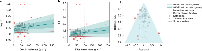
Following Zheng et al.20, we modeled each non-linear dose–response as a quadratic spline21. For each risk–outcome pair, we first modeled the non-linear RR function without a monotonicity constraint to observe the unconstrained behavior. For outcomes in which the mean curve remained above one across the whole domain and was generally increasing, we then fitted a final model applying a monotonicity constraint to ensure that the mean risk curve was non-decreasing. For outcomes in which the curve decreased then increased and was minimized at a non-zero value, we did not apply a monotonicity constraint but instead implemented a linear-tail constraint (sometimes referred to as ‘natural’ splines in curve-fitting literature) on the left side of the domain to ensure more plausible risk curve behavior at low exposure levels. Linear-tail constraints ensure that the final segment on one side of the domain is linear, rather than a quadratic or cubic binomial and are a common way to regularize spline behavior. We present the sensitivity of the results based on this assumption in the Supplementary Information, section 2.1.
Because knot placement can affect the shape of the risk function when modeling with a spline, we generated a wide range of knot placements and created an ensemble across 50 component models, weighted by their fit to the data and the smoothness of fit to the observations. We also included in the final estimation 10% trimming of the data to avoid sensitivity to outliers; trimming from within the likelihood is an efficient way to identify outliers without manually selecting them21,105. Through this process, we generated a mean RR curve across the range of exposures (a measure of effect size) for each red meat–outcome pair. We obtained uncertainty estimates for the mean risk curves using a parametric bootstrap approach. Details on the fitting procedure, including trimming, ensemble generation and posterior uncertainty estimation, can be found in Zheng et al.20.
Testing for bias across different study designs and characteristics
To capture bias within the studies and data points, we followed the approach of Zheng et al.20, using a Lasso106,107 covariate selection scheme to rank the potential bias covariates. We then converted the dose–response relationship previously estimated by non-linear meta-regression into a new ‘signal’ covariate and used linear meta-regression to systematically test for significant modification of the ‘signal’ by each bias covariate—adding them to the model one at a time based on the Lasso ranking. Significant bias covariates were then included in the spline models; the details of this procedure have been published elsewhere20. Supplementary Information, section 3 provides more information on our risk of bias assessment.
Quantifying between-study heterogeneity, accounting for heterogeneity, uncertainty and small numbers of studies
The variance of between-study random effects is notoriously difficult to estimate. We quantified between-study heterogeneity (the level of disagreement in the inferred relationship between risk and outcome found in each study) by scaling the non-linear RR based on each study using a study-specific random slope with respect to the new bias covariate model. For cases with small numbers of studies, the estimated between-study heterogeneity can often be zero. To safeguard against underestimating the between-study heterogeneity when too few studies were available, we used the Fisher information matrix108 to estimate the variance of the between-study heterogeneity, Zheng et al.20 provides more details. Our main results include the effect of between-study heterogeneity in UIs, although we also present UIs that do not include it (as is standard in conventional meta-regressions) in Supplementary Table 7.
Evaluating potential for publication or reporting bias
To assess potential publication or reporting bias, we used a data-driven approach known as Egger’s regression109 to test for significant correlation between the residuals of the risk function and their s.d. When Egger’s regression failed to detect significant evidence of publication bias, we terminated the process.
When significant bias was detected, we adjusted for it using an appropriate modification of the trim-and-fill algorithm110. The trimming process in extracting the signal covariate is robust both to outliers and to classic cases of publication bias. Given a robust estimate of the mean curve, we applied the ‘fill’ part of the trim-and-fill approach, using the rank statistics and residuals to compute the number of points that need to be ‘filled’. The correct number of the most extreme residuals was then reflected and might affect our resulting estimate of heterogeneity. When fitting for the updated between-study heterogeneity, we used a prior coming from the original fit, with s.d. obtained from the Fisher information.
In addition to this statistical test of publication or reporting bias, we generated funnel plots of the residuals of the risk function and s.d. and inspected them visually. In the presence of significant publication bias, we used the trim-and-fill method to adjust for bias20,110.
Determining minimum risk consumption level
To determine the minimum risk level of red meat consumption, we aggregated the outcome-specific risk curves to generate an aggregated mortality curve for the six causes in our analysis combined, which we used to identify the exposure range that minimizes risk. Specifically, we took a weighted average of the risk curve draws for each outcome, using the GBD 2019 burden of each outcome—with deaths as the metric—as weights5,111. Then we calculated the exposure level that minimized combined-cause mortality for each draw and reported the median and associated 95% UI.
Estimating the burden of proof risk function
Using estimates of the mean risk function and corresponding 95% UIs—inclusive of between-study heterogeneity and reflective of other bias adjustments—as described in the preceding sections, we calculated a BPRF for each risk–outcome pair. Specifically, for γ = between-study heterogeneity, we let γ 0.95 represent the 95% quantile according to the asymptotic distribution obtained using Fisher information. We computed the lower envelope of the log-RR curve that included fixed effects uncertainty as well as γ 0.95 and found the average value of this curve at specific exposures and along the specified ranges of exposure. The BPRF is defined as the fifth (if harmful) or 95th (if protective) quantile risk curve—inclusive of between-study heterogeneity—closest to the RR equal to one (the null). The BPRF reflects a conservative interpretation of the available evidence and is a measure of the lowest level of excess risk (or risk reduction, for protective risks) that is consistent with the available data; the higher the BPRF, the higher the magnitude and strength of the relationship. This value can be interpreted such that even accounting for between-study heterogeneity and its uncertainty, we are confident that the log RR across the studied unprocessed meat consumption range is at least as high as the BPRF (or at least as low as the BPRF for a protective risk).
We then calculated ROSs as the signed average log RR of the BPRF over the 15th to 85th percentiles of observed exposure20. For example, a mean log BPRF of 0.4 for a harmful risk (where null = 0 for log RR) and a mean log BPRF of –0.4 for a protective risk would both have an ROS of 0.4 because the magnitude of the log RR is the same. In contrast, for risk–outcome pairs with a BPRF opposite the null from the mean risk, ROS would be calculated as negative. A positive risk score indicates that across average levels of exposure, the UI bound that is closest to null is on the same side of null as the mean risk curve. Positive ROSs indicate evidence of a risk–outcome relationship. Overall, a larger positive ROS indicates more consistency in evidence and a higher average effect size across the continuum of the risk. As an estimate of strength of evidence, the ROS is also directly comparable across outcomes, so we can use it to rank disease outcomes by confidence in their relationship to red meat consumption.
Finally, to aid interpretability of our findings for policy makers and research funders, we converted the ROSs to star-rating categories from one to five, with a higher rating indicating that the evidence for and magnitude of a relationship between risk and outcome is stronger. The conservative interpretation suggests that, for one-star pairs, there may be no true association between risk exposure and health outcome. As noted, we further divided the positive ROSs into ranges of at least a 0–15% increase (for harmful risks) or 0–13% decrease (for protective risks) in risk with average exposure (two stars), >15–50% increase or >13–34% decrease (three stars), >50–85% increase or >34–46% decrease (four stars) and greater than 85% increase or greater than 46% decrease (five stars). In ROS terms, the ranges are <0.0, 0.0–0.14, >0.14–0.41, >0.41–0.62 and >0.62 for both harmful and protective risks.
Model validation
We used detailed simulations to validate key components of the meta-regression model. The details of these model validations are available in Zheng et al.20. In brief, we simulated three scenarios: many studies with many data points per study, many studies with few data points per study and few studies with few data points per study. For each simulation, we compared the results from our model with results obtained using existing approaches, including a log-linear meta-analysis implemented in the metafor package112 as well as one-stage113 and two-stage114 competing approaches using the dosresmeta package115. For log-linear relationships, our approach and the metafor package showed similarly superior performance over the one- and two-stage approaches, whereas for non-log-linear relationships, our approach produced uniformly better performance across all scenarios compared to the other approaches.
Statistical analysis
Analyses were carried out using R v.3.6.1, Python v.3.8 and Stata v.17. To validate key aspects of the meta-regression model used in this analysis, the following packages were used, as described by Zheng et al. metafor (R package available for download at https://www.jstatsoft.org/article/view/v036i03) and dosmesreta (R package available for download at https://www.jstatsoft.org/article/view/v072c01).
Statistics and reproducibility
The study was a secondary analysis of existing data involving systematic reviews and meta-analyses. No statistical method was used to predetermine sample size. As the study did not involve primary data collection, randomization, blinding and data exclusions are not relevant to this study; and, as such no data were excluded and we performed no randomization or blinding. We have made our data and code available to foster reproducibility.
Reporting summary
Further information on research design is available in the Nature Research Reporting Summary linked to this article.