Study design and participants
We sought to test our hypothesis and predictions using the Personalized Responses to Dietary Composition Trial (or “PREDICT1”). PREDICT1 is a single-arm, single-blind intervention study, whose overall objective is to understand glucose, insulin, lipid and other postprandial responses to foods based on the individual’s characteristics, including molecular biomarkers, lifestyle factors, in combination with the nutritional composition of the food. The official start and end dates for the study were 5 June 2018 and 8 May 2019, the first participant was enrolled on 4 August 2018 and the last clinical visit was completed on 24 April 2019, with the primary cohort based at King’s College London in the UK and a second cohort (that underwent the same profiling as in the UK) assessed at Massachusetts General Hospital in Boston, MA, USA. In the UK, participants (target enrollment, 1,000 participants) were recruited from the TwinsUK cohort, a prospective cohort study, and online advertising. In the USA, participants (target enrollment, 100 participants) were recruited through online advertising and research participant databases. The written informed consent and ethical committee approvals covered all analysis reported in the current study in addition to the key primary outcomes described in9. The trial was registered on ClinicalTrials.gov (registration number: NCT03479866 , first posted on March 27, 2018) as part of the registration for the PREDICT program of research, which also includes two other study protocol cohorts (not analysed in the current study). The trial was run in accordance with the Declaration of Helsinki and Good Clinical Practice. The study was approved in the UK by the Research Ethics Committee and Integrated Application System (IRAS 236407) and in the US by the Institutional Review Board of Partners Healthcare (Protocol # 2018P002078). Participants did not receive financial compensation for taking part in the study.
Study participants were healthy individuals aged 18–65 years, who were able to provide written informed consent. Exclusion criteria included ongoing inflammatory disease; cancer in the last three years (excluding skin cancer); long-term gastrointestinal disorders including irritable bowel disease or Celiac disease (gluten allergy), but not including irritable bowel syndrome; taking immunosuppressants or antibiotics as daily medication within the last three months; capillary glucose level of >12 mmol l–1 (or 216 mg dl–1), or type 1 diabetes mellitus, or taking medication for type 2 diabetes mellitus; currently experiencing acute clinically diagnosed depression; heart attack (myocardial infarction) or stroke in the last 6 months; pregnancy; and vegan or experiencing an eating disorder or unwilling to consume foods that are part of the study. Diagnosis or symptoms of any sleep disorders, circadian rhythm disorders, or neurocognitive disorders were not exclusionary. Similarly, the use of medication to impact sleep, circadian or brain function was not exclusionary.
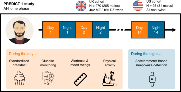
A total of 970 generally healthy adults from the United Kingdom (including non-twins, monozygotic [MZ] twins and dizygotic [DZ] twins) as well as 95 healthy adults from the United States (all non-twins) were enrolled and completed baseline clinic measurements, as well as a two-week at-home phase. For more details on the clinic measurements, we refer the reader to the online protocol8.
During the study’s home-phase, participants consumed multiple standardised test meals differing in macronutrient composition (carbohydrate, fat, protein and fibre), while wearing a physical activity monitor. Standardised meals were consumed at breakfast during the first 9-11 days of the home period, and additionally for lunch on the two first days. Participants recorded their dietary intake and alertness on the Zoe study app throughout the study. Following completion of the home-phase, participants returned all study samples and devices to study staff via standard mail.
Data collection and analysis
For an exhaustive description of all the outcomes measured in the PREDICT1 study, we refer the reader to the full online protocol8. Briefly, key outcomes included postprandial metabolic responses (blood triglyceride, glucose, and insulin concentrations) to sequential mixed-nutrient dietary challenges administered in a tightly controlled clinical setting on day 1. A second set of outcomes was assessed over the subsequent 13 d at-home period. Primary outcomes include gut microbiome profile, blood lipids and glucose, sleep, physical activity, and hunger and appetite assessment. The main analysis of the primary outcomes has been reported elsewhere8,52. The current study reports a non-preregistered/exploratory analysis of the association between the secondary outcome of subjective alertness and the primary outcomes of sleep, physical activity, diet, and blood glucose (all measured during the at-home phase of the study). Data from the UK and US sub-cohorts were combined into a single dataset in the current study.
Questionnaires
Data on socio-demographic characteristics, medical health, habitual diet, and lifestyle were collected via a self-administered baseline questionnaire during the clinic visit. Education. Academic education was measured on a scale from 0 (no qualifications) to 8 (postgraduate degree). Subjective sleep. Subjective sleep quality was assessed using the well-validated Pittsburgh Sleep Quality Index (PSQI)53. The PSQI measures 7 domains of sleep quality over the past month to provide a global score (0-21) of overall sleep quality, with higher scores indicating poorer sleep quality. In addition, participants were asked to report their typical bedtime and waketime, in both weekdays and weekends. The absolute difference between the midpoint of sleep in weekdays and weekends was then used to quantify social jetlag54, with higher values indicating a greater mismatch between an individual’s own biological rhythm and the daily timing determined by social constraints (assuming that most individuals worked during the weekdays and did not work during the weekend). Habitual diet and eating behaviours. Habitual diet was measured using the European Prospective Investigation into Cancer and Nutrition (EPIC) food frequency questionnaire (FFQ) in the UK cohort and the Harvard semi-quantitative FFQ in the US cohort. The questionnaire also included questions related to eating frequency (“how many times do you eat in a day?”), habitual coffee and alcohol consumption, and whether the participants usually skip breakfast. Exercise. Self-report exercise frequency was measured with the following question: “In the past year, how frequently have you typically engaged in physical exercises that raise your heart rate and last for 20 minutes at a time?” Mental health. Current/former clinical diagnosis of depression and anxiety disorder was measured using the following questions: “Has a doctor ever told you that you have/had any of the following conditions? [clinical depression, anxiety or stress disorder]”.
Standardised test meals
Upon completion of their baseline visit, participants received a home-phase meal pack containing test-meals varying in macronutrient composition, which they consumed according to standardised instructions for breakfast and, on some days, lunch. Test meals consisted of either an oral glucose tolerance test (OGTT) or muffins, which were consumed on their own or paired with chocolate milk, a protein shake or commercial fibre bars. The description and nutritional composition of the test meals can be found in Table 1. Test meals were consumed in a different order depending on which protocol group participants were assigned to, as described in the online protocol8. Test meals were prepared and packaged in the Dietetics Kitchen (Department of Nutritional Sciences, King’s College London). As is common practice for postprandial studies55, meal sizes were similar across all participants and not normalised by weight or total daily energy expenditure.
Participants were instructed to fast for a minimum of 8 hours prior to consuming a test breakfast meal (i.e., avoid nighttime snacking), and to fast for 3 or 4 hours after the test meal consumption. Furthermore, they were advised to limit exercise and drink only plain, still water during the fasting periods. When fasting was completed, participants could eat, drink and exercise as they liked for the rest of the day. Participants were asked to consume all muffin-based meals within 10 minutes and the OGTT within 5 minutes, and to notify study staff if this was not achieved, in which case the data were excluded from the analysis.
If the participant chose to accompany their home-phase muffin-based test meals with a tea or coffee (with up to 40 ml of 0.1% fat cow’s milk, but without any sugar or sweeteners), they were instructed to consume this drink consistently, in the same strength and amount, alongside all muffin-based test meals throughout the study. Participants were instructed to not consume any food or drink other than water alongside the OGTT. They recorded test meals and any other dietary intake within fasting periods, including accompanying drinks in the study app (see next section) with the exact time of consumption and ingredient quantities so that study staff could monitor compliance. Only test meals that were completed according to instructions were included in the analysis.
Food and alertness logging via mobile study app
The Zoe study app was developed to support the PREDICT 1 study by serving as an electronic notebook for study tasks. The app sent participants notifications and reminders to complete tasks at certain time-points, such as when their test lunch meals were due. Participants logged their full dietary intake using the study app over the 14-day study period, including all standardised test meals and free-living foods, beverages (including water) and medications.
Data logged into the app was uploaded onto a digital dashboard in real time and reviewed and assessed for logging accuracy and study guideline compliance by study staff. The Zoe study app contained a database of generic and branded food items with nutritional information sourced from generic data sources, commercial food databases under licence, back-of-pack information from commercial providers, and publicly available restaurant nutritional data. It also allowed participants to photograph back of pack labels in cases where this information was missing from the nutritional database, and where possible, the photographed information was entered into the database by study staff.
The app also prompted participants to report their alertness levels on a visual analogue scale56 by displaying the question “how alert are you?”. These app notifications appeared at t = 0 (time of logging) and regular intervals (+0.5, +1.5, +2.5 hours) following the logging of a breakfast, lunch or dinner meal. However, given the free-living conditions of the study, participants did occasionally miss one or more ratings, resulting in a variable number of alertness ratings per day per participant. The app also prompted participants to report their happiness and anxiousness levels once per day at ~9 PM local time. Here again, a visual analogue scale was used with the following question: “How have you been feeling generally over the whole day: How happy have you felt”?
For both the meals and alertness data, participants with less than 5 days of valid data were removed (n = 56 [5.3%] and n = 42 [3.49%] participants excluded, respectively). Second, participants that travelled in a different timezone during the two weeks of the home-based study were also excluded (n = 65 [5.59%] participants). Data regarding travel to a different time zone in the weeks before the study was not available.
Postprandial glucose
Interstitial glucose was measured every 15 min using Freestyle Libre Pro CGMs (Abbott). Monitors were fitted by trained nurses on the upper, non-dominant arm at participants’ baseline visit and were covered with Opsite Flexifix adhesive film (Smith & Nephew Medical) for improved durability, and were worn for the entire study duration. The 2 hours incremental area under the curve (2hr-iAUC) was used for analysis of the postprandial glucose response9. The distribution of glucose 2hr-iAUC was skewed and the data was thus transformed using a Yeo-Johnson power transformation.
Sleep/wake
Sleep/wake patterns were measured using a triaxial accelerometer (AX3, Axivity, Newcastle Upon Tyne, UK). The accelerometer was fitted by clinical practitioners at the baseline clinic visit on the non-dominant wrist and worn for the duration of the study (except during water-based activities, including showers and swimming), after which they were removed on day 15 and mailed back to study staff. The accelerometer was programmed to measure acceleration at 50 Hz with a dynamic range of ±8 g (where g refers to the standard acceleration of gravity, i.e., approximately 9.81 m/s2). Non-wear periods were defined as windows of at least 1 hour with less than 13 mg for at least 2 out of 3 axes, or where 2 out of 3 axes measured less than 50 mg57.
Raw accelerometer data was analyzed using the “GGIR” R package version 1.10-758. Sleep/wake detection was then quantified using the validated algorithm described in ref. 49, which uses the variance in the accelerometer z-axis angle together with a set of heuristic rules to determine sleep periods. This algorithm does not require a sleep diary and has been validated against gold-standard polysomnography in both healthy individuals and patients with sleep disorders, with a mean concordance statistic of 0.86 and 0.83, respectively49. For each night and each participant, the following sleep metrics were calculated (see Fig. 1): sleep onset, sleep midpoint, sleep offset, sleep duration (defined as the elapsed time from sleep onset through sleep offset, or sleep period time [SPT]), wake after sleep onset (WASO), total sleep time (TST; = SPT - WASO), sleep efficiency (SE, = TST / SPT). SE was calculated using the SPT and not the more common total time in bed as denominator because the absence of sleep diary data precludes the accurate estimation of bedtime prior to sleep. For the same reason, the algorithm is unable to characterise sleep onset latency (the time between going to bed and falling asleep). The GGIR algorithm is not able to detect naps and therefore only nighttime sleep parameters were included in subsequent analyses.
A set of thresholds was then applied to remove invalid nights or participants, consistent with typical practices59. First, any nights with a TST outside the range of 2 to 15 hours, or a SE below 20%, was excluded (376 nights, 2.5%). Second, nights with more than 10% classified as invalid were excluded (403 nights, 2.65%). Third, nights with a sleep onset between 8 AM and 5 PM or a sleep offset after 12 PM were excluded (45 nights, 0.3%). Finally, participants with less than 5 days of valid sleep data (n = 60, 5.53%) were removed, consistent with the preprocessing of the food and alertness data.
Physical activity
Physical activity was measured using the accelerometer and features were calculated, for each day and each participant, using the GGIR software. Specifically, these features consisted of the M10 and L5 values, and their associated onset timings. M10 and L5 refer to the most-active 10 hours and the least-active five hours of each day, respectively, and are commonly studied measures relating to circadian activity10,59. The M10 was defined as the 10-h period with the maximum average acceleration, estimated using a 10 hours moving average. The L5 was defined as the 5-h period with the minimum average acceleration, estimated with a 5-hours moving average. For these two metrics, the onset timings was also calculated, defined as the number of hours elapsed from the previous midnight. Once again, participants with less than 5 days of valid physical activity data were removed (n = 51, 4.72%).
Data concatenation
Sleep, meal (including postprandial glucose), physical activity and alertness data were all merged into a single dataframe to facilitate statistical analyses. Here, a strict inner-merge was performed, meaning that only the participants and days with valid food, physical activity, alertness and sleep data were included in the final dataframe. The sleep and physical activity features were shifted by one day to ensure a valid temporal directionality, i.e., that sleep/physical activity occurred before, and not after, the alertness outcome.
A final quality check was applied that consisted of removing, for each day and each participant, the alertness ratings that were logged one hour or more before the algorithm’s predicted sleep offset (916 ratings, 1.0%). Concretely, this removes the alertness ratings that were input before sleep and after midnight (as these should technically be counted for the previous day).
Statistical analyses
Multilevel modelling
Linear mixed-effects models were used to measure the statistical association of sleep, food intake and its associated glucose response, and physical activity with subsequent alertness. Unless specified otherwise, all multilevel models were adjusted for age, sex, body mass index (BMI), twin status (MZ, DZ or NT), sunrise time, daylight saving time (DST), and weekend (i.e., whether the day on which the person wakes up is a Saturday or Sunday); with family identifier and subject identifier defined as nested random effects.
Income, work schedule (including shift work) and household size were not available in PREDICT1 and therefore the statistical models could not be adjusted for those.
To account for the natural between-person variability in sleep, the sleep predictors — duration, efficiency and waketime — were normalised using person-mean centering. That is, they were expressed, for each participant separately, as a deviation from this individual’s average calculated across the two weeks of the study.
All multilevel analyses were performed in R60 using the “lme4”, “lmerTest”,“sjPlot” and “emmeans” packages61,62,63,64. Goodness-of-fit was evaluated with the conditional \({R}^{2}\)65. For all multilevel models, the variance inflation factor (VIF) was used to check for multicollinearity. When multicollinearity was detected (VIF > 5), the correlated predictors were removed from the model and/or split into two separate multilevel models66. Diagnostic plots were used to assess the validity of the fitted models. For each multilevel model, these included scatterplots of standardised residuals by fitted values and observed versus fitted values. Normal quantile plots (Q–Q plots) were used to check the assumption of normality of the residuals and random effects.
The performance of the multilevel model in predicting new, unseen data was then tested using a hold-out validation. This step is increasingly recommended to prevent overfitting and improve the interpretability of the findings67. The dataset was separated into a training and testing set, based on a split of odd and even days (e.g. training = days 1, 3, 5, …; testing = days 2, 4, 6, …). Importantly, the assignment of odd days to the training or testing set was randomly decided for each participant. Then, a multilevel model was fitted on the training set, using the same predictors and random effects as the main model. The resulting regression coefficients were then used to make predictions on the testing set. Performance was evaluated using the coefficient of determination (r-squared) between the true and predicted alertness values. All statistical tests reported in the manuscript are two-tailed.
Machine-learning analysis of the trait predictors of alertness
For between-person (i.e., trait) analysis of alertness, a machine-learning approach was used to evaluate the relative importance of a large number of trait measures on alertness. These predictors included: the age, sex, education level, smoking status, BMI, average sleep and physical activity parameters calculated across the two weeks of the study, self-report measures of subjective sleep quality (PSQI score) and social jetlag, self-report happiness, self-report habitual amount of exercise, self-report medical diagnosis of depression or anxiety disorder, and self-report eating behaviours — including whether or not the participant usually skip breakfast, habitual coffee and alcohol consumption, eating frequency and snacking.
Several of these parameters were highly correlated and/or contained missing values. For these two reasons, the association of these predictors with alertness could not be evaluated using a standard regression approach, which would have resulted in a dramatic decrease in sample size as well as invalid regression coefficients because of multicollinearity. Addressing these issues, a gradient boosting machine-learning algorithm (LightGBM,11) was used as the primary analytical method for the between-person analysis. Gradient boosting algorithms are based on decision trees and are therefore robust to multicollinearity in predictors. In addition, they natively support missing values, without the need for deletion or imputation. The LightGBM model was trained with 50 estimators and a random subsampling of all features and samples (50%) before building each tree. Performed of the model on unseen data was evaluated using a 3-fold cross-validation of the full dataset.
Next, Shapley values were used to assess the unique contribution of each feature in predicting trait alertness. Shapley values have several desirable properties that make them ideal to evaluate the unbiased feature importance of the predictors of a statistical model. Specifically, they quantify, for each observation (i.e., participant), the exact impact of a given feature — after accounting for all other features — on the outcome of the model. Shapley values were first computed for each feature and each participant using the SHAP library68. Global feature importance was then calculated by averaging the absolute Shapley values of a given predictor across all observations.
All machine-learning algorithms were conducted in Python using the “scikit-learn”, “lightgbm“, “shap” and “pingouin” packages11,68,69.
Heritability analyses
A large proportion of the main cohort consisted of pairs of identical (MZ) and fraternal (DZ) twins, which allows a test of genetic influences upon alertness and sleep inertia. For each dependent variable, we first calculated the intra-pair correlation separately for MZ and DZ siblings. The former share the vast majority of their germline DNA sequence70, while the latter are assumed to share on average 50% of their segregating genetic material. DZ twins are, however, presumed to share their common environmental influences (e.g. family) to the same extent as MZ twins. Therefore, the degree to which MZ siblings have a higher correlation for a specific trait than DZ siblings reflects the extent of genetic influence on this trait.
Heritability was then calculated using a standard twin model71, which decomposes the observed phenotypic variation into a combination of additive (A) and non-additive (D) genetic variance, common environmental variance (C; familial influences that contribute to twin similarity) and individual-specific environmental variance plus measurement error (E). The combination of these factors that best matches the observed data is found with structural equation modelling techniques. Because the C and D factors are negatively confounded, they cannot be estimated simultaneously. Therefore, following standard guidelines, an ACE model was used when the DZ twin correlation was more than half the MZ twin correlation, and an ADE model otherwise. The broad heritability (\({h}^{2}\)) was then defined as the percentage of total phenotypic variance that could be explained by genetic factors (= A in ACE models and A + D in ADE models).
The significance of genetic factors (A and/or D) was assessed by means of likelihood ratio tests comparing the full model with a nested model in which these factors were constrained to be zero. When the fit significantly worsened, the contribution of genetic factors was considered significant. Finally, the Akaike Information Criterion (AIC) was used to determine the best-fitting model, with lower AIC indicating a better fit of the model to the observed data.
All heritability analyses were conducted using the “mets” R package72. Twin models were adjusted for age and sex. To account for repeated measurements in the twin models, analyses focused on the participants’ grand-averaged values73.
Reporting summary
Further information on research design is available in the Nature Portfolio Reporting Summary linked to this article.