Toilet Rig
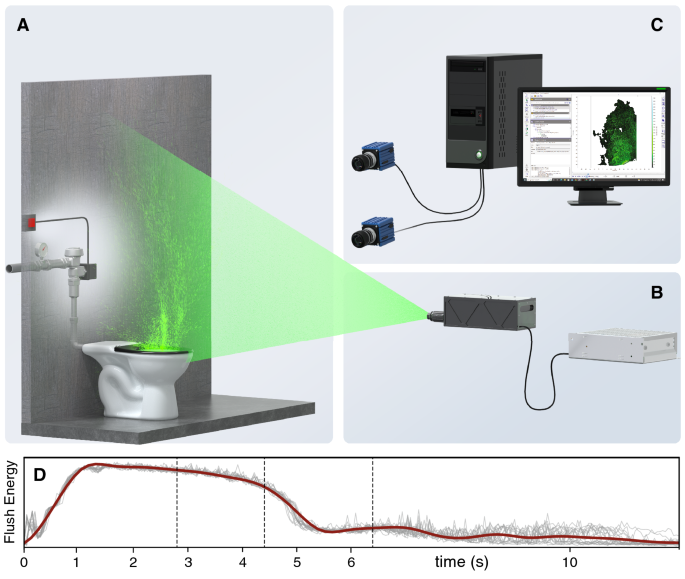
To measure toilet aerosol plumes in our laboratory, we use a commercial toilet with a common 1.6 gallon-per-flush flushometer-style valve, typical of those found across North America in public restrooms. The toilet is fitted with a commercial seat in the “down” position that is painted flat black to minimize laser reflections. There is no lid fitted to the toilet, consistent with most commercial toilet installations. The rear of the toilet abuts a solid wall; the flushometer valve and associated plumbing are behind this wall.
An electric pump fills a 14 gal water tank with an internal pre-charged air bladder system; the pump is set to shut off when the tank pressure reaches 60 psi, at which point the toilet is ready to be flushed (the flushometer valve has a recommended supply pressure between 10 and 100 psi). The tank is plumbed to the flushometer inlet, and the flush cycle is initiated via a remote button that activates a solenoid on the flushometer valve. During the flush, pressure in the tank drops ‘such that the supply pressure at t = 7.5 s (final panels in Figs. 3 and 4) has dropped to 45 psi. Following the flush cycle and data acquisition, the pump is activated to reset the tank pressure to 60 psi. The experiments are performed in an open laboratory space, and we rely on the laboratory HVAC system to ventilate flush-generated particles between experiments.
Imaging with continuous laser
To capture color images (Figs. 2 and 6) and video (Movie S1) of the aerosol plume, we use a continuous wave (CW) laser (IPG Photonics GLR-50, 532 nm wavelength, operating at a power level of 11 W) to illuminate a vertical plane aligned with the toilet’s axis of symmetry. Light sheet optics spread the beam into a sheet with a 2 mm beam waist centered on the field of view (FOV). Mie scattering of laser light by aerosol particles is imaged with a Sony camera (a6300) fitted with a Sony 50 mm f/1.8 lens. Still images are acquired with a 1/50 s shutter speed at 4000 x 6000 pixel resolution, and videos are acquired at 60 fps with 1/60 s shutter speed and 1920 \(\times\) 1080 pixel resolution.
While our imaging technique is most effective at imaging the location and motion of larger aerosols (5-10 \(\mu\)m) that scatter more light, post-processing the images to increase brightness and reduce contrast (Fig. 6) demonstrates that it is also able to capture dimmer light scattered by smaller aerosols, and that the smaller particles move within the same envelope as the larger ones.
Figure 6 Imaged particles are good indicators of the plume envelope. (A) The third panel of the plume (t = 6.4 s) from Fig. 2 is reproduced here for reference, showing the location and motion of larger particles. (B) Enlarged image of the region denoted by the red box in part A, post-processed to increase exposure and decrease contrast. This renders dimmer light from smaller particles visible, and demonstrates that the smaller particles (green glow) are well predicted by the locations of larger particles (imaged as discrete points of light). Also visible in the lower left are several large droplets that are following ballistic trajectories and are outside the aerosol plume envelope. Full size image
Imaging with pulsed laser
To quantify the spatiotemporal evolution and kinematics of flush-induced aerosol plumes (Figs. 3, 4) we use a dual-cavity, double-pulsed Nd:YAG laser (Quantel EverGreen 200, 532 nm wavelength, operating at 200 mJ/pulse). The laser emits pairs of pulses (\(dt=\) 2.25 ms), each with a 5 ns pulse width. Pulse pairs are repeated at 15 Hz. As with the CW laser, we use sheet optics to create a 2 mm light sheet spanning the FOV. Images are acquired using two sCMOS cameras (LaVision Imager sCMOS; 16-bit monochrome, 2160 \(\times\) 2560 pixel resolution) fitted with Nikkor 50 mm f/1.2 lenses. The cameras are stacked vertically (Fig. 1C), with the long axis of the sensors oriented vertically and pointed such that there is a 15% overlap in the FOV of each camera; this permits individual images to be stitched together to provide a combined FOV (0.57 m wide \(\times\) 1.23 m high) that is large enough to capture the entire toilet plume during the first 8 s following flush initiation, with a spatial resolution of 260 \(\mu\)m/pixel. The narrow depth-of-field associated with the f/1.2 lens aperture, along with the thin light sheet and 5 ns illumination pulses permits selective imaging of scattered light from in-sheet aerosols for subsequent computation of plume envelopes and aerosol velocities.
A large spatial calibration target consisting of a high-contrast square grid covering the entire FOV of the combined camera set is used (i) to compute the optical magnification of the imaging system, (ii) to reference the image data to the toilet geometry in physical space, and (iii) to map each camera to a common point in physical space, allowing for the accurate stitching of the two individual FOVs into a single data image covering the total resolved FOV. The known geometry of the grid on the calibration plate is also used to create a pinhole model32 to dewarp the individual camera images, correcting for potential image distortions associated with small oblique imaging angles and/or lens distortions. The pinhole model is appropriate for our planar imaging configuration with undisturbed optical access through air. The estimated uncertainty in the reconstructed/combined image data is less than 0.5 px.
Closely-spaced (2.25 ms separation) pairs of images are acquired from each camera at a rate of 15 Hz during flush events. The images are used to quantify the spatiotemporal evolution of the plume envelope (Fig. 3) and to compute aerosol velocities (Fig. 4) using particle image velocimetry30, 31, 33. All laser and camera timing sequences and associated image acquisition, storage, and processing are achieved on a high-performance computer running DaVis 10.2 software (LaVision GmbH).
Imaging system resolution
For the 260 \(\mu\)m/pixel resolution of our optical system (described above), individual aerosol particles (0.1 \(\mu\)m - 10 \(\mu\)m) are only a small fraction of the imaged size of an individual pixel. However, for our low-magnification optical system, aperture diffraction34, 35 causes the imaged size of these aerosol particles to increase to at least a theoretical minimum of approximately 0.25 pixel, regardless of their physical size. Then, lens aberrations further enlarge the theoretical minimum diffraction size by as much as an order of magnitude, particularly for systems with large working distances (> 1 m) as is the case for ours (\(\approx\) 2 m). Digitization and quantization of the continuous particle image signal onto a discrete pixel grid can also enlarge the recorded particle size. Thus, individual aerosol particles are expected to produce imaged spots that are several pixels or more in diameter. Furthermore, given that the true size of individual aerosol particles is tiny compared to the pixel resolution of our system, it is reasonable to expect that the light gathered by a single pixel is due to a large number of particles, all of which contribute to the imaged intensity at that point. Consistent with these arguments, our recorded images exhibit strong particle images with typical diameters \(d_D\) of 1.5 to 4 pixels (see PIV section below). The result is that the strong multi-pixel images of particles (or even large numbers of particles) are well suited for instantaneous mapping of the spatial envelope of the aerosol plume (Fig. 3) and computing aerosol velocities (Fig. 4). However, the same optical properties that render the optical system suitable for these tasks preclude its use for counting and sizing of individual aerosols. For this reason, counting and sizing are done separately with the airborne particle counter (Fig. 5).
Generation of plume envelopes
The spatial extent of the aerosol plume envelope is computed from image data using a simple two-step image processing algorithm commonly used in PIV applications to delineate seeded and unseeded regions. First, a sliding maximum filter is applied to fill in regions of low pixel intensity between individual particle images. With appropriate filter length selection, the effect is to both increase and homogenize pixel intensities inside the plume envelope with minimal effect on regions outside the plume. Then a global intensity threshold is used to identify the in-plume versus out-of-plume regions (since higher pixel intensities correspond most notably to the presence of plume aerosols, as well as the size and local density of aerosols). While large changes in the tuning parameters produce local artifacts (e.g., unwarranted internal voids, or excessive perimeter smoothing), the general shape and spatial extent of the plume is generally robust for a range of tuning parameters.
Determination of velocity fields with PIV
Particle image velocimetry (PIV) is used to compute aerosol velocities inside the detected plume envelope33. Here, each sCMOS camera acquires double-frame image data, where pairs of images are acquired at the imaging frequency of 15 Hz, which sets the temporal resolution of the velocity measurements. The image pair itself is separated by a short time dt, the cross-correlation timescale of the PIV analysis. A near-optimal dt results in maximum particle image displacements of approximately 8–10 px for a 32 px correlation subwindow ( the “1/4-rule” of37) based on the optical magnification of the imaging system and the physical velocities associated with particles. Here, a dt of 2.25 ms (set by the time delay between laser pulse pairs) is effective at resolving the high velocities (1 - 2 m/s) associated with the strong vertical jet that develops early in the flush cycle (Fig. 3) and minimizing the associated velocity uncertainty.
Particle signal level relative to background (intensity counts), particle seeding density (particles per pixel), and particle image diameter (pixels) strongly influence the resolved dynamic velocity range (DVR)36. Our imaging configuration yields signal levels (post background subtraction) of 8–10 bits ensuring good particle fidelity and strong intensity correlations. Seeding densities are set by the spatiotemporally evolving local density of aerosol clouds (and limitations of the imaging system resolution described above) and typically range between 0.001 and 0.02 ppp within the plume envelope. These densities span the commonly-accepted value of 0.01 ppp, sufficient to provide strong cross-correlation peaks and acceptable uncertainty levels. Finally, typical particle image diameters of \(d_D=\) 1.5 to 4 px are sufficient to alleviate “peak locking” effects (integer pixel displacements) when implementing window-shifting correlation techniques as described below38. Image sets are first pre-processed to remove background artifacts and to enhance particle fidelity. Aerosol displacement (velocity) fields are then computed using modern digital correlation and interrogation techniques described below. Image preprocessing, PIV correlation analyses, and vector postprocessing are achieved on a high-performance computer running DaVis 10.2 software (LaVision GmbH).
Aerosol velocity fields (Fig. 4) are computed from image pairs via cross-correlation of intensity patterns within small interrogation subwindows inside the detected plume envelopes. Best practices are used to maximize the measurement DVR including multi-pass iterative schemes with overlapping (50% - 70%) subwindows of decreasing sizes (96 px - 32 px), adaptively shaped to local flow conditions. The resulting vector fields are then post-processed using an imposed minimum correlation peak ratio (1.4) to detect outliers and noisy vectors, which are discarded. The peak ratio is the ratio of the strongest correlation peak to the next strongest in a given interrogation window, and correlates well with the estimated measurement error39, providing a proxy for the effective DVR of the measurement. Finally, any gaps in the post-processed vector fields are filled using spatial interpolation and nonlinearly smoothed to preserve local gradients. The resulting vector field is space-filling inside the plume envelope with a spatial resolution of 2.08 mm/vector. Typical maximum local velocity uncertainties are less than 5% of the local velocity magnitude and rarely approach 10% (estimated using correlation statistics40). Corresponding peak ratios typically exceeding 10 throughout the plume envelope confirm the high DVR and good fidelity of the aerosol velocity measurements.
In traditional PIV applications, low Stokes number particles are introduced into the flow as passive tracers (“seeding particles”) whereas here we use the aerosols themselves to serve as natural tracers. The Stokes numbers (St = ratio of particle inertial timescales to the advection timescales of the flow) of 1-micron particles in the highest-velocity portions of the plume (around 1 m/s) are O(1). While larger aerosols around 10-micron exhibit higher St in these regions, the predominantly vertical velocities associated with the strong jet suggest that aerosol clouds of the sizes of interest here (0.1 - 10 microns) behave acceptably as passive tracers. The implication of all of the above for the PIV-based velocity is as follows: individual velocity vectors represent the mean velocity averaged over small clouds of aerosols (producing individual particle images on the sensor) and over collections of discrete aerosol clouds (producing all the particle images contained in a PIV interrogation subwindow).
Sound measurements
As a metric for flush duration and intensity we acquire sound pressure levels with dB(A) frequency weighting using a Google Pixel 3 smartphone with a pre-calibrated mobile application (Decibel X, SkyPaw Co., Ltd.). Twenty replicates of a 12 second interval surrounding the flush cycle are recorded, where \(t=0\) corresponds to when the flush button is pushed. The average sound pressure profile shown in Fig. 1D is smoothed with a cubic B-spline, downsampling by a factor of 10 to capture the characteristic shape. A second spline was applied with the original number of samples for smoothing.
Airborne particle counting
Particle counting is done with a portable airborne particle counter (Particle Measuring Systems HandiLaz Mini II) suspended in the locations shown in Fig. 5A. The counter is sensitive to particles ranging in size from \(0.2\ \mu\)m (d50) to \(10\ \mu\)m, and outputs counts in 60 discrete logarithmically-spaced bins across this range. For clarity, we grouped particle counts from the instrument into the three broader bins shown in Fig. 5; particle sizes larger than \(2.5\ \mu\)m are not shown since these counts were close to zero. The counter ingests 2.83 liters/min, and the nozzle is oriented downwards, since the plume was generally approaching from below. For each location, particles are counted over three 37 s intervals (Fig. 5B). Each interval consists of five 5s samples separated by 3 s periods when the data is written to storage. The timing of the intervals at location 3 differs slightly from those in locations 1 and 2 due to phase differences in the discrete sampling by the instrument. Five replicates are acquired, with average and arithmetic standard deviations reported in Fig. 5C.