Participants
For experiment 1, a total of 58 healthy participants including 30 younger adults (aged between 19 and 30 years), and 28 older adults (aged between 65 and 78 years) with corrected-to-normal vision and no history of neurological, psychiatric disorder or alexithymia took part. Thirty individuals were expected to participate in each group; however, new research guidelines during the coronavirus disease 2019 pandemic prevented us from continuing with scanning. Recruitment was performed through social media and advertisement in various locations within the University of Geneva. Three participants were excluded due to a priori exclusion criteria, including artifacts in brain images and/or extreme head motion during scanning. The final sample for experiment 1 included 29 young participants (mean age, 24 years; 14 females) and 26 older participants (mean age, 68.7 years; 13 females), resulting in a total of N = 55 participants (see Table 1 for detailed participant characteristics). All participants provided written informed consent. This study was approved by the local Swiss ethics committee (Commission Cantonale d’Ethique de la Recherche CCRE, Geneva) under project number 2018–01980.
For experiment 2, a total of 137 healthy older adults participated, community-dwelling, with corrected-to-normal vision and no history of neurological or psychiatric disorders, aged between 65 and 83 years. This session was part of the baseline visit of the Age-Well randomized controlled trial (RCT) within the Medit-Ageing Project70, conducted in Caen (France). Detailed inclusion criteria of the Age-Well RCT are provided in Supplementary Table 1. Participants were recruited via advertising in media outlets, social media and flyers distributed at relevant local events and locations. Two participants were excluded for eligibility criteria and intervention allocation issues71. A total of 8 participants were excluded from the final data analysis due to a priori exclusion criteria, including abnormal brain morphology (n = 3), extreme head motion (n = 3) and presence of artifacts in brain images (n = 2). The final sample for this study included 127 participants (mean age, 68.8 years, s.d. 3.63 years; 79 females; see Table 1 for other characteristics). All participants provided written informed consent before participation. The Age-Well RCT was approved by the ethics committee (Comité de Protection des Personnes Nord-Ouest III, Caen, France; trial registration number: EudraCT, 2016-002441-36; IDRCB, 2016-A01767-44; ClinicalTrials.gov identifier: NCT02977819).
Questionnaires
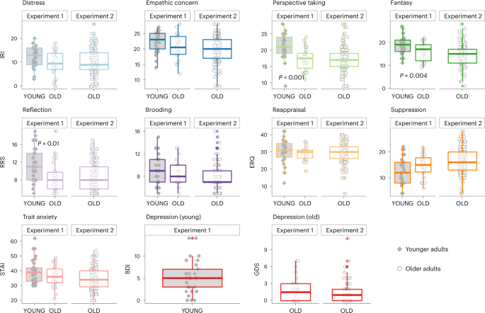
To account for interindividual differences in psycho-emotional profile, all participants from both experiments answered several questionnaires assessing psycho-affective traits and cognitive functions, including empathy (IRI72), depression (GDS73 for older adults and BDI74 for younger adults), anxiety (State-Trait Anxiety Inventory, STAI75), emotion regulation capacities (ERQ76) and rumination levels (RRS77). A summary of these questionnaires is provided in Table 1 and Fig. 1. All scores were in the normative range. For a full list of tasks and measures in the Age-Well trial (experiment 2), please refer to Poisnel and colleagues70.
Socio-affective video task–rest
The emotion-elicitation task used in both experiments was adapted from the previously validated SoVT43,45. The SoVT aims to assess social emotions (for example, empathy) in response to short silent videos (10–18 s). During this task, participants watch 12 HE and 12 LE video clips grouped in blocks of three (see instructions in Supplementary Table 2). HE videos depict people suffering (for example, due to injuries or natural disasters), while LE videos depict people during everyday activities (for example, walking or talking). In this study, each block was followed by a resting-state period of 90 s (see instructions in Extended Data Fig. 1 and Supplementary Table 2) to assess the carryover effects of emotion elicitation on subsequent resting-state brain activity (similar to Eryilmaz and colleagues17). This combination of both paradigms (task and rest) was specifically designed to test for emotional inertia and its relation to empathy. The combined task (SoVT–rest) is illustrated in Extended Data Fig. 1.
Overall, three sets (V1, V2 and V3) of 24 videos each were created and randomized across participants. In experiment 1, the video sets V1, V2 and V3 were seen by n = 21, 18 and 16 participants, respectively. In experiment 2, these were seen by n = 42, 40 and 45 participants, respectively. In both experiments, these videos were presented in two separate runs, always followed by a rest period. In experiment 2, each run was followed by a thought probe to assess current mental content during the last rest period (after LE videos in one run and after HE videos in the other run). The order in which runs were presented was randomized so that half of the participants started the experiment with a HE block and the other half with an LE block. No thought probe was given in experiment 1 (as it primarily aims at determining age-related brain activity patterns at rest). Brief instructions (in French) were presented before each period within each block. These indicated ‘The task is about to start’ before the first period of videos, or ‘The next videos are going to start’ before those in the following periods; while the display ‘Rest: wait for the next videos’ appeared before each rest period (Extended Data Fig. 1a,b). The total duration of the SoVT–rest fMRI paradigm was approximately 21 min, consisting of 9.5 min for each run, plus 1 min on average for the thought probes.
After the fMRI session, participants watched all video clips again on a computer outside the scanner and provided ratings on their subjective experience of empathy (‘To what degree did you feel the emotions of the characters?’) as well as their subjective positive affect (‘Indicate the intensity of your positive emotions’) and negative affect state (‘Indicate the intensity of your negative emotions’; translated from French), for each of the 24 videos. Each scale offered 21 possible responses ranging from 0 (‘not at all’) to 10 (‘extremely’) with increments of 0.5. The order of questions was always the same: empathy, positive affect and negative affect. We chose to obtain ratings after fMRI not only to minimize the time older adults spent in the scanner, but also to avoid potential cognitive effects during scanning that may confound neural activity during emotional perception and spontaneous rest recovery periods68,78. The total time for post-scanning ratings was, on average, 10 min. Onset times and response times for both neuroimaging and behavioral tasks were collected via the Cogent toolbox (developed by Cogent 2000 and Cogent Graphics) implemented in MATLAB 2012 (MathWorks).
Acquisition and preprocessing of magnetic resonance imaging data
Experiment 1
MRI scans were acquired at the Brain and Behavior Laboratory of the University of Geneva, using a 3T whole-body MRI scanner (Trio TIM, Siemens) with the 32-channel head coil. A high-resolution T1-weighted anatomical volume was first acquired using a magnetization-prepared rapid acquisition gradient echo (MPRAGE) sequence (repetition time, 1,900 ms; echo time, 2.27 ms; flip angle, 9°; slice thickness, 1 mm; field of view, 256 × 256 mm2; in-plane resolution, 1 × 1 mm2). Blood oxygen level-dependent (BOLD) images were acquired with a susceptibility-weighted EPI sequence (TR/TE, 2,000/30 ms; flip angle, 85°; voxel size, 3 × 3 mm; 35 slices, 3-mm-slice thickness, 20% slice gap; direction of acquisition, descending). Quality control and preprocessing were conducted using Statistical Parametric Mapping software (SPM12; Wellcome Trust Centre for Neuroimaging) on MATLAB 2017 (MathWorks). Before preprocessing, we manually centered all images to the AC-PC axis, aligned the functional and anatomical MRI images, and then realigned all images to the SPM anatomical template. Preprocessing included the following steps: (1) EPI data were realigned to the first volume and spatially smoothed with an 8-mm FWHM Gaussian kernel; (2) preprocessed fMRI data were denoised for secondary head motion and cerebrospinal fluid-related artifacts using automatic noise selection as implemented in ICA-AROMA, a method for distinguishing noise-related components based on ICA decomposition79. Additionally, components with high spatial overlap with white-matter regions were also removed by means of a linear regression using the fsl_regfilt function of FSL 6.0 (FMRIB’s Software Library; https://fsl.fmrib.ox.ac.uk/fsl/fslwiki/); (3) denoised EPI data were co-registered to the anatomical T1 volume; (4) the anatomical T1 volume was segmented and the extracted parameters were used to (5) normalize all EPI volumes into the Montreal Neurological Institute space. This procedure was performed using FSL and SPM12.
Experiment 2
MRI scans were acquired at the GIP Cyceron using a Philips Achieva 3T scanner with a 32-channel head coil. Participants were provided with earplugs to protect hearing, and their heads were stabilized with foam pads to minimize head motion. A high-resolution T1-weighted anatomical volume was first acquired using a three-dimensional fast field echo sequence (3D-T1-FFE sagittal; repetition time, 7.1 ms; echo time, 3.3 ms; flip angle, 6°; 180 slices with no gap; slice thickness, 1 mm; field of view, 256 × 256 mm2; in-plane resolution, 1 × 1 mm2). BOLD images were acquired during the SoVT–rest task with a T2*-weighted asymmetric spin-echo echo-planar sequence (each run ~10.5 min; TR, 2,000 ms; TE, 30 ms; flip angle, 85°; FOV, 240 × 240 mm2; matrix size, 80 × 68 × 33; voxel size, 3 × 3 × 3 mm3; slice gap, 0.6 mm) in the axial plane parallel to the anteroposterior commissure. During each functional run, about 310 contiguous axial images were acquired and the first two images were discarded because of saturation effects. Additionally, to improve the preprocessing and enhance the quality of the BOLD images80, T2 and T2* structural volumes were collected. Each functional and anatomical image was visually inspected to discard susceptibility artifacts and anatomical abnormalities.
Quality control and preprocessing were conducted using statistical parametric mapping software (SPM12; Wellcome Trust Centre for Neuroimaging) on MATLAB 2017 (MathWorks). Before preprocessing, we manually centered the images to the AC-PC axis, realigned the functional and anatomical MRI images and then realigned all images to the last version of the SPM anatomical template. The preprocessing procedure was done with SPM12 and followed a methodology designed to reduce geometric distortion effects induced by the magnetic field, described by Villain and colleagues80. This procedure included the following steps: (1) realignment of the EPI volumes to the first volume and creation of the mean EPI volume; (2) co-registration of the mean EPI volume and anatomical T1, T2 and T2* volumes; (3) warping of the mean EPI volume to match the anatomical T2* volume, and application of the deformation parameters to all the EPI volumes; (4) segmentation of the anatomical T1 volume; (5) normalization of all the EPIs, T1 and T2* volumes into the Montreal Neurological Institute space using the parameters obtained during the T1 segmentation; (6) 8-mm FWHM smoothing of the EPI volumes.
For each individual, frame-wise displacement (FD)81 was calculated. FD values greater than 0.5 mm were flagged to be temporally censored or ‘scrubbed’ during the first-level analysis (see description below). The average of FD volumes censored was 6.8 (s.d. 8.3, minimum of 1, maximum of 38) for both runs for a total of n = 65 participants. Three participants were excluded from further analysis because >10% of volumes showed FD > 0.5 mm within one run.
General linear model analysis
For both experiments, the MRI SoVT–rest data were analyzed using GLMs in SPM12 (implemented in MATLAB 2017). This comprised standard first-level analyses at the subject level, followed by random-effect (second-level) analyses to assess the effects of interest at the group level. For the first-level analysis, a design matrix consisting of two separate sessions was constructed for each participant. Experimental event regressors in each session included the fixation cross (10 s), instructions (8 s in experiment 1, 4 s in experiment 2), the three videos (~15 s each) modeled separately, and the rest periods following each block (90 s). Each rest period was divided into three equal parts (30 s time bins) to model different time intervals during which brain activity may gradually change after the end of the HE and LE video blocks (similar to Eryilmaz and colleagues17).
The different regressors were then convolved with a hemodynamic response function according to a block design for univariate regression analysis. To account for motion confounds, the six realignment parameters were added to the matrices, and low-frequency drifts were removed via a high-pass filter (cutoff frequency at 1/256 Hz). The final first-level matrix consisted of 2 sessions of 21 regressors each (1 fixation cross + 1 instruction for videos + 1 instructions for rest + 3 HE videos + 3 post-HE rest + 3 LE videos + 3 post-LE rest + 6 motion parameters). Additionally, we addressed the influence of remaining motion on BOLD data by performing data censoring as described by Power and colleagues81. Specifically, during the estimation of beta coefficients for each regressor of interest, volumes with FD > 0.5 mm were flagged in the design matrices and ignored during the estimation of the first levels.
For the second-level analyses, we used flexible factorial designs where the estimated parameters from first-level contrasts of interest were entered separately for each participant. The second-level design matrix was generated with SPM12 and included 12 regressors of interest (3 HE videos + 3 post-HE rest + 3 LE videos + 3 post-LE rest). This step allowed us to investigate the effect of each experimental condition on brain activity, including the main condition effects (video and rest), the specific emotional effects (HE and LE) during either the video or the subsequent rest periods as well as the age effect on the different conditions (young versus old; experiment 1).
Functional connectivity during rest periods
For both experiments, we conducted functional connectivity analyses between the most important brain ROIs associated with the empathy network and with the DMN. In addition, we also included the bilateral amygdalae among regions used for this analysis because previous studies assessing carryover effects in the brain have related sustained amygdala activity to anxiety traits15 and emotional reactivity61. For nodes of the DMN, we chose the PCC and the aMPFC, following Andrews-Hanna and colleagues59. Based on the results of a meta-analysis by Fan and colleagues39, the bilateral AI and aMCC were used as ROIs in the empathy network. Time series were extracted from 6-mm-radius spheres around the peak of each of these ROIs. The amygdala was defined anatomically using the current SPM anatomical template provided by Neuromorphometrics (http://neuromorphometrics.com/).
Functional connectivity analyses were performed using MATLAB 2017 and R studio (version 3.6.1). For each participant, time courses of activity (from each voxel of the brain) were high-pass filtered at 256 Hz, de-trended and standardized (z-score) before extracting specific time courses from the defined ROIs. In addition, white matter, cerebrospinal fluid signals, and realignment parameters were included as nuisance regressors in experiment 2. For each participant, time series from the instructions and videos periods were removed, and the remaining time series corresponding to the rest periods were concatenated. This procedure was previously proposed by Fair and colleagues82 and proved to be qualitatively and quantitatively very similar to continuous resting-state data. Additionally, to correct extreme head motion without affecting the autocorrelation of the time series, image volumes flagged with FD > 0.5 mm were removed and replaced by interpolation (every flagged volume X was replaced by the estimated mean of the X − 1 and X + 1 volumes). The final concatenated time series resulted in 184 frames (∼386 s) of resting-state data for each participant. We then correlated the time courses between the different ROIs using Pearson correlations, and the resulting coefficients were subjected to Fisher’s r-to-z transformation to improve normality in the data. Individual z-score maps (correlation matrices) were created for each participant (Extended Data Fig. 2a,b,c).
Thought probes
For each participant in experiment 2, two thought probes were recorded after the last rest period of each run and subsequently analyzed to test for differences in spontaneous mind wandering after emotional videos. Participants freely described their thoughts, and these narratives were digitally recorded and transcribed for analyses by two independent raters (Supplementary Table 4). For each probe (post-HE rest and post-LE rest), the two raters attributed the presence (present) or the absence (absent) of specific thought contents according to a diverse set of predefined categories (Supplementary Table 4). These categories were selected according to a priori relevant affective or cognitive dimensions, and included the following: negative and positive emotions, directed attention to oneself and to others, emotion regulation (voluntary control of emotions), negative and positive social emotions, rumination and temporality (present or past/future). Categories with low variability (that is, the same thought content reported by more than 85% of participants) were not included in further analyses because this prevented reliable regression analysis (Supplementary Table 4). The final dimensions included negative and positive emotions, directed attention to oneself and to others, and positive social emotions. This final analysis of thought probes comprised data from 109 participants for rest periods after HE videos and 110 participants for the rest periods after LE videos. This was due to (1) missing thought probes for 9 participants and (2) exclusion of reports not referring directly to thoughts or feelings in the rest period (but rather to factual details in the videos) for both runs (n = 5), following LE rest (n = 3) or following HE rest (n = 4). Inter-rater agreement on the final dimensions ranged from 0.28 to 0.66 (Cohen’s kappa index; Supplementary Table 4 for details). The statistical analyses were performed with R studio (version 3.6.1) and the corresponding graphs were created with ggplot2 (version 3.2.1).
Statistics and reproducibility
Statistical analyses of behavioral data
We performed a repeated-measures multivariate analysis of variance (with Pillai’s trace statistics) with the within-subject factor ‘video type’ (HE and LE), the between-subject factor ‘video set’ (V1, V2 and V3) and three dependent variables: ratings of empathy, positive affect and negative affect. This was followed up by pairwise t-tests. We also computed Spearman’s rank correlations between these different scores. Additionally, we performed correlation analyses between ratings of empathy, positive affect and negative affect of videos and age (as a continuous variable), using non-parametric Spearman’s rank correlations because some of these variables were not normally distributed. All statistical analyses are reported with a significance level of P < 0.05, and when necessary, P values were corrected for multiple comparisons using the FDR method83. Normality in the data was tested, and non-parametrical tests (for example, Spearman’s rank correlations) were performed when estimated necessary.
Statistical analyses of brain activity
In both experiments, we conducted t-tests contrasts to compare the conditions of interest (videos versus rest periods and vice versa) and the specific emotional effects (videos, HE versus LE; rest, HE versus LE). In experiment 1, we additionally tested for age differences in these effects (OAs versus YAs (videos, HE versus LE); OAs versus YAs (rest, HE versus LE)). In experiment 1, results are reported at uncorrected P < 0.001, k > 20 because this dataset concerned a smaller sample size and aimed at defining a comprehensive set of brain regions with emotion-related modulations in either videos or rest period in either age group. These regions could then be further probed with higher reliability and related to relevant individual characteristics in the larger dataset of experiment 2. Moreover, a more permissive combination of voxel-based and cluster-based thresholds has been shown to be adequate and reliable for experiments assessing cognitive and affective processes with unprecise onsets84, as in our task–rest paradigm. In addition, we had strong predictions concerning relevant regions (for example, DMN) based on previous works17,24,43. Finally, clusters surviving whole-brain family-wise error correction at P < 0.05 at the cluster level (FWEc) in experiment 1 are indicated in figures and tables (Supplementary Table 3a). In experiment 2, all comparisons are reported with a whole-brain FWE correction at P < 0.05, at the voxel level (Supplementary Table 3b).
Statistical analyses of brain functional connectivity
To test for significant differences between the two correlation matrices (post-HE rest and post-LE rest), we used a non-parametric permutation test85. For each pair of nodes, the permutation test compared the true correlation difference (for example, HE − LE) to a null distribution built by randomly flipping the sign of the correlation coefficients and computing the difference many times (n = 5,000; Extended Data Fig. 2d). More precisely, for each pair of nodes (for example, HE − LE for ROI 1 and ROI 3), a vector of values of n = number of participants was obtained and a one-sample t-test was computed to obtain the real t value (t real ). Then, the signs of the elements in the vector were randomly flipped (n = 5,000) and the model was fitted repeatedly once for every flipping. For each fit, a new realization of the t-statistic was computed to construct an empirical distribution of t under the null hypothesis (t permuted ). From this null distribution, a P value was computed by assessing the probability of the t real to be higher than 95% of the values on the empirical t permuted distribution85. Finally, the obtained P values were converted into an equivalent z-score and significant changes (marked by an asterisk in matrices) were retained for z > 1.64 (equivalent to P < 0.05, one-tailed, given observed increases without decreases in GLM analysis, uncorrected).
The final sample for experiment 1 included N = 55 participants. Three participants were excluded due to a priori exclusion criteria, including artifacts in brain images and/or extreme head motion during scanning. No statistical methods were used to predetermine sample sizes but our sample sizes are similar to those reported in previous publications17,35. The final sample for experiment 2 included N = 127 participants. Two participants were excluded for eligibility criteria and intervention allocation issues71. Eight participants were excluded from the final data analysis due to a priori exclusion criteria: abnormal brain morphology (n = 3), extreme head motion (n = 3) and presence of artifacts in brain images (n = 2). For the primary outcome of the Age-well RCT, an effect size of 0.75 per comparison was targeted, with 80% power and a two-sided type I error of 1.25% (Bonferroni correction for test multiplicity), resulting in a total of 126 participants needing to be included. The final number of participants in the Age-Well RCT (n = 137) was higher than the required minimum of 126 participants70,71. Sensitivity analyses then indicated that the final sample included in experiment 2 (n = 127) was reliable and sensitive enough to detect small- to medium-sized effects at a voxel level (α = 0.001, effect size of dz = 0.37), given a power of 1 − ß = 0.8 (ref. 86). For both experiments, the video sets (V1, V2 and V3) and whether participants started the experiment with HE or LE videos first were randomly attributed to participants in an Excel table. While investigators were blinded to the training arm that participants were randomized to in the Age-Well trial, no blinding was performed for the SoVT–rest task at baseline (experiment 2). The statistical analyses were performed with R studio (version 3.6.1) and MATLAB 2017 (MathWorks), and the corresponding graphs were created with ggplot2 (version 3.2.1).
Reporting summary
Further information on research design is available in the Nature Portfolio Reporting Summary linked to this article.