Study site
The fieldwork was conducted in the Jemez River Basin Critical Zone Observatory (JRB-CZO) within the Valles Caldera National Preserve in the Jemez Mountains in north-central New Mexico45 (Supplementary Fig. 1). The JRB has an elevation of 1700-3432 m a.s.l., and at its upper elevations it contains montane mixed-conifer forests that are common high-elevation ecosystems throughout the western United States. The study site is a mature forested low-gradient hillslope that drains into a first-order channeled basin45. This study site was established in the fall of 2015. It contains an instrumented flux tower (Ameriflux) and three instrumented pedons located ~20 m from the flux tower (Supplementary Fig. 1). Canopy heights range from 10 to 31 m around the flux tower. The three pedons were excavated and instrumented in August 2015 (Supplementary Fig. 1). The parent material of the soils is rhyolitic tuff.
The Jemez Mountains are located in the transition zone between southwestern US and the snow-dominated Rocky Mountains46,47. Thus, the Jemez Mountains have a bimodal pattern of annual precipitation, with approximately half of annual precipitation falling as winter snow, and the other half as rain45. This region has a typical semiarid and montane climate with annual precipitation ranging from 600 to 1021 mm and mean annual precipitation of 777 mm. Air temperature at the study site ranges from –15 °C in the winter to 25 °C in the summer, with average winter and summer temperatures of ~–1 °C and 11 °C.
Meteorological measurements and monitoring of soil microclimate
Flux tower-based meteorological measurements of above-ground ecosystem-atmosphere exchanges of water and energy fluxes have been conducted since January 2016 in the ZOB (Ameriflux Site ID: US-Vcs). Here, we focus only on data of precipitation, net radiation (NETRAD), and gross primary production (GPP, which is equivalent to apparent photosynthesis, i.e., net ecosystem exchange minus ecosystem respiration). Meteorological measurements enable correlation between above- and below-ground processes.
Co-located sensor and sampler instruments were installed in the instrumented pedons (Fig. 2). Soil moisture and temperature were quasi-continuously monitored at depths of 2, 10, 30, 60, and 135 cm within the three instrumented soil pits (located ~20 m from the AmeriFlux tower) from October 2015 to October 2017. These data were measured at 15 min intervals and were stored in CR1000 dataloggers (Campbell Scientific, Logan, Utah, USA). Soil moisture and temperature were measured using Decagon 5TE sensors (Decagon Devices Inc., Pullman, Washington, US).
Measurement of soil O 2 and CO 2 partial pressures
Partial pressures of soil O 2 and CO 2 were continuously measured at 2, 10, 30, and 60 cm within the three pedons using Apogee SO-110 (galvanic cell) and solid-state infrared gas sensors GMP-222 (Vaisala Inc., Helsinki, Finland), respectively. Partial pressures of soil CO 2 (P CO2 ) recorded by the sensor were corrected for variations in pressure and temperature48 as follows:
$${C}_{c}={C}_{m}-{C}_{P}-{C}_{T}$$ (1)
where C represents the partial pressure of CO 2 , and the subscripts c, m, P, and T represent corrected, measured, pressure correction, and temperature correction, respectively. The atmospheric pressure-corrected P CO2 , C p , was calculated as:
$${C}_{P}={K}_{P}\left[\frac{P-101.3}{101.3}\right]$$ (2)
where P (kPa) is the atmospheric pressure recorded by flux tower and K P (ppm) was calculated as:
$${K}_{P}=1.38\times {C}_{m}$$ (3)
The temperature-corrected P CO2 , C T , was calculated as:
$${C}_{T}=14000 \, ({K}_{T}-{K}_{T}^{2})\left[\frac{25\,-\,{T}_{c}}{25}\right]$$ (4)
where Tc is the soil temperature (°C) and K T (ppm) was calculated as:
$${K}_{T}={{{{{{\rm{A}}}}}}}_{0}+{{{{{\rm{A}}}}}}_{1}\times {C}_{m}+{{{{{\rm{A}}}}}}_{2}\times {{C}_{m}}^{2}+{{{{{\rm{A}}}}}}_{3}\times {{C}_{m}}^{3}$$ (5)
with A 0 = 3 × 10⁻³ ppm, A 1 = 1.2 × 10⁻⁵, A 2 = –1.25 × 10⁻⁹, A 3 = 6 × 10⁻¹⁴.
Similarly, partial pressures of soil O 2 (P O2 ) were also corrected for variations in pressure and temperature.
Calculation of soil CO 2 efflux
We used the gradient method, which is based on the gradient of soil CO 2 concentration and effective CO 2 diffusivity of the soil to calculate soil CO 2 efflux48,49. The CO 2 flux (F) at a depth of z can be calculated using Fick’s first law of diffusion:
$${F(z)}={-}{{{{{{\rm{D}}}}}}}_{s}\frac{{dC}}{{dz}}$$ (6)
where D s is the effective CO 2 diffusivity within the soil (m2 s−1), \(\frac{d{{{{{\rm{C}}}}}}}{d{{{{{\rm{z}}}}}}}\) the vertical CO 2 gradient, and the negative sign indicates that the efflux is decreasing upwards. C (μmol m−3) here can be converted from corrected P CO2 (μmol mol−1) by:
$${C}=\frac{{C}_{c}P}{{{{{{\rm{R}}}}}}T}$$ (7)
where R is the universal constant (8.314 J mol−1 K−1), T the soil temperature (K), and P the air pressure (Pa). D s can be calculated as:
$${D}_{s}=\xi {{{{{{\rm{D}}}}}}}_{a}$$ (8)
$${{{{{{\rm{D}}}}}}}_{a}={{{{{\rm{D}}}}}}_{a0}\left(\frac{T}{293.2}\right)^{1.75}\left(\frac{101.3}{P}\right)$$ (9)
where D a is the CO 2 diffusion coefficient in the air, D a0 a reference constant (1.47 × 10⁻⁵ m2 s−1) at 101.3 kPa and 293.2 K, and ξ the gas tortuosity factor. Several models have been proposed for computing ξ, and we chose the model by Moldrup et al.50 (2000) for our samples because it often produces results in good agreement with chamber-based estimates:
$${{{{{\rm{\xi }}}}}}=\frac{{({{{{{\rm{\varphi }}}}}}-{{{{{\rm{\theta }}}}}})}^{2.5}}{{{{{{\rm{\varphi }}}}}}}$$ (10)
where φ represents the porosity, and θ the volumetric water content. The difference between these two parameters is equal to air-filled porosity (ε):
$${{{\rm{\varphi }}}}={{{{{\rm{\varepsilon }}}}}}+{{{{{\rm{\theta }}}}}}=1-\frac{{\rho }_{s}}{{\rho }_{m}}$$ (11)
where ρ s is the bulk density of the analyzed soil, and ρ m is the particle density of the mineral soil, with an assumed value of 2.65 g cm−3. Combining these equations, we can calculate CO 2 flux (f CO2 ) at depth z (F(z)).
Calculation of water flux
Soil water flux at each soil depth can be directly calculated from passive capillary sampler (PCAP) datasets. The PCAPs, which are passively collecting water flux data at all times, are excellent for calculation of water flux because of the nature of the hanging water column. From those PCAPs, we calculated the volume of water passing through the soil profile per unit area to get water flux data. Specifically, water flux (f H2O ) was calculated by dividing the volume collected in the PCAP carboy by the cross-sectional area of the PCAP plate (7.8 × 10⁻² m2), which gives the volume flux of water for the period of collection (T) that contributes to recharge:
$${f}_{{{\rm{H2O}}}}=V/(T\times 7.8\,\times {10}^{-2}{{{{{{\rm{m}}}}}}}^{2})$$ (12)
Solute flux (e.g., f SO4 and f DIC ) was calculated by multiplying solute concentration (e.g., [SO 4 2−] and [DIC]) by water flux. Because water flux was calculated using integrated data for a whole year, we generated only a single water flux datum for a specific depth. However, water flux should fluctuate through each year due to temporal variability in rainfall and soil moisture content. Thus, we also multiplied solute flux by soil moisture to get moisture-corrected solute flux data (e.g., f SO4-corr and f DIC-corr ).
Collection of soil-porewater and precipitation samples
Soil porewaters were collected in situ weekly or biweekly throughout the rainy season (March to October) during 2016 and 2017 and for more limited intervals during 2018 and 2019. They were collected with two types of soil porewater samplers, i.e., Prenart Super Quartz tension lysimeters (2 μm pore size, Prenart Equipment ApS, Denmark) and fiberglass wick-based passive capillary wick samplers (PCAPs51). These samplers have proven effective for soil porewater sampling and suitable for analysis of DOM51. The Prenart Super Quartz tension lysimeters were installed at depths of 10, 30, 60, and 135 cm, and the PCAPs were installed at depths of 10, 30, 60 cm in each soil pit. These installations provided vertically and temporally resolved porewater samples. For Prenart Super Quartz tension lysimeters, a vacuum pump applied a constant suction of 40 kPa to collect soil solution samples into high-density polyethylene (HDPE) bottles. PCAPs consist of a fiber-glass wick covered with a HDPE plate. PCAPs were used to collect soil solutions as a function of depth in each pit under a constant negative pressure head of ~30 cm (~2.9 kPa). Precipitation samples were collected on 15 March 2015 from four snowpacks (with samples taken at three depths within each snowpack) near the flux tower and three soil pits.
Soil-porewater and precipitation chemistry analyses
All soil-porewater and precipitation samples were kept frozen and sent overnight to the University of Arizona Laboratory for Emerging Contaminants to be filtered within 48 h of collection using 0.45 μm nylon filters. Sample aliquots for DOM and DIC were filtered through combusted 0.7 μm glass-fiber filters. Concentrations of DOC ([DOC]) and DIC ([DIC]) were determined by infrared detection of CO 2 after catalysis at 720 °C (DOC) or aridification (DIC) using a Shimadzu TOC-VCSH carbon analyzer (Columbia, MD). DIC, an important parameter in this study, was defined as the sum of H 2 CO 3 aq (carbonic acid), [HCO 3 −], [CO 3 2−], and soil CO 2 , which would react with porewater to form DIC:
$${{{{{{{\rm{CO}}}}}}}_{2}}^{{{{{{\rm{gas}}}}}}}+{{{{{{\rm{H}}}}}}}_{2}{{{{{\rm{O}}}}}} \, \rightleftharpoons \, {{{{{{\rm{H}}}}}}}_{2}{{{{{{{\rm{CO}}}}}}}_{3}}^{{{{{{\rm{aq}}}}}}} \, \rightleftharpoons \, {{{{{{\rm{H}}}}}}}^{+}+{{{{{{{\rm{HCO}}}}}}}_{3}}^{-} \, \rightleftharpoons \, 2{{{{{{\rm{H}}}}}}}^{+} \,+\, {{{{{{{\rm{CO}}}}}}}_{3}}^{2-}$$ (13)
where H 2 CO 3 aq represents the hydrated form of dissolved CO 2 .
The speciation of Eq. (13) is mediated by soil porewater pH: for a soil pH < 6.4, H 2 CO 3 * dominates DIC, with HCO 3 − dominating at 6.4 < pH < 10.352. Per Henry’s law, the amount of dissolved CO 2 in water is proportional to the soil P CO2 :
$${{P}_{{{\rm{CO2}}}}}^{{{{{{\rm{gas}}}}}}} \, \rightleftharpoons \, {K}_{H}\times [{{{{\rm{CO}}}}_{2}}^{{{{{{\rm{aq}}}}}}}]$$ (14)
$$[{{{{{{{\rm{CO}}}}}}}_{2}}^{{{{{{\rm{aq}}}}}}}]+{{{{{{\rm{H}}}}}}}_{2}{{{{{\rm{O}}}}}} \, \rightleftharpoons \, {{{{{{\rm{H}}}}}}}_{2}{{{{{{{\rm{CO}}}}}}}_{3}}^{{{{{{\rm{aq}}}}}}}$$ (15)
where K H represents Henry’s law constant for CO 2 (34.06 mol m−3 atm−1) at 25 °C. Henry’s law implies that DIC can reflect the P CO2 in soil pore spaces and thus the intensity of microbial decomposition of SOM to DOM via soil heterotrophic respiration.
Concentration of dissolved nitrogen ([DN]) was measured by nitrate colorimetric analysis after high-temperature combustion of all N species to nitrate. We assume that inorganic N is mainly present in the form of NO 3 −, and thus the concentration of dissolved organic nitrogen ([DON]) can be calculated as the difference between [DN] and the concentration of NO 3 –N. Concentrations of anions (e.g., Cl−, NO 3 −, and SO 4 2−; abbreviated as [Cl−], [NO 3 −], and [SO 4 2−], respectively) were analyzed by ion chromatography using Dionex ICS-1000 equipped with an AS22 Analytical Column, Sunnyvale, CA. Concentrations of cations and silicon were determined by ICP-MS (ELAN DRC-II, Shelton CT).
Soil porewater inorganic chemistry data were used to perform aqueous geochemical modeling with MINTEQ3.1. The modeling involves determination of aqueous phase speciation and calculation of SI values of pore waters with respect to various potentially precipitating secondary phases. The SI was calculated as:
$$SI={{{\rm{log}}}}\,\varOmega={{{\rm{log}}}} \, IAP \, {-} \, {{{\rm{log}}}}\,{K}_{sp}$$ (16)
where Ω is the relative saturation, IAP is the ion activity product, and K sp is the solubility product constant at a given temperature. Positive SI specifies supersaturation and precipitation of the solid, and negative SI specifies undersaturation and dissolution. DOC concentration and site density (2.4 × 10⁻⁶ mol of sites per mg DOC) were used as input parameters to account for metal-ligand complex formation.
Plotting of time series
Time series of mineralogical and organic and inorganic geochemical parameters were plotted for four depths within the instrumented pedons (10, 30, 60 and 135 cm) using filtered data. For each sampling date, data for the three pedons are spread out slightly on the temporal axis for display purposes—for example, data for 4/19/2016 are plotted as 4/18/2016 for pit 1, 4/19/2016 for pit 2, and 4/20/2016 for pit 3. Because the distribution of sampling dates is uneven, we used a ‘homogenization’ function in Excel to make the plots more uniform, rendering the dates on the x-axis unevenly distributed but improving the visual aspect of the plots. These graphical transformations did not alter any data in the porewater geochemical dataset. In a few cases (e.g., time series of total cation charge, Sr/Ba and f SO4 ), mean values were used to better compare information conveyed in different types of plots.
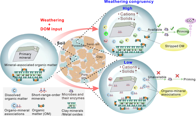
Calculation of weathering congruency and priming effect
Products of congruent weathering are only dissolved species, whereas products of incongruent weathering also contain solid phases (Table 1). The relative contribution of weathering congruency vs. incongruency can be measured by normalizing element release to that of dissolved sodium53, which is considered a “conservative” tracer of mineral dissolution, because it does not re-incorporate into secondary solid structures, and it is a weak competitor for cation exchange sites. Here we use the ratio of {[Si] solution /[Na] solution }/{[Si] solid /[Na] solid } (simplified as [Si]/[Na] norm ) to provide a normalized measure of weathering stoichiometry (weathering congruency). The priming effect caused by fresh DOM input can be quasi-quantitatively estimated by comparing f DIC-corr and f CO2 before and after the introduction of “fresh” DOM during the period with very minor change in weathering congruency (Supplementary Fig. 12):
$${Absolute}\,{P}{{E}}_{{DOM}}={Respons}{{e}}_{^{{\prime\prime}} {fresh}^{\prime\prime}} {DOM} \, {-} \, {Respons}{{e}}_{^{{\prime\prime}} {control}^{\prime\prime} }$$ (17)
$${Relative}\,{P}{{E}}_{{DOM}} (\%)=\frac{{Response}_{^{\prime\prime} {fresh}^{\prime\prime}} {DOM} -{Response}_{^{\prime\prime} {control}^{\prime\prime}} }{{Response}_{^{\prime\prime} {control}^{\prime\prime}} }\times 100$$ (18)
where Response “fresh” DOM and Response “control” represent f DIC-corr (mg C m−2 yr−1) and f CO2 (μmol m−2 s−1) after and before the input of more bioavailable (“fresh”) DOM, respectively. The criteria for selection of the period of the priming-effect calculation is a notable increase in FI (microbial activity) accompanied by diminishing SUVA 254 (increasing bioavailability) with minor variation in weathering congruency, as this kind of period may represent a “fresh” DOM-induced priming process. Thus, f DIC-corr and f CO2 at the beginning of this period can be viewed as a control group for the calculation of the priming effect at different depths.
After calculating the priming effect at different depths, we quantify the influence of mineral weathering on the priming effect. For a specific soil depth, we view the period with relatively low [Si]/[Na] norm values as a “control group” with low weathering congruency. It is worth noting that the priming effect in the control group was not unimpacted by chemical weathering but it had almost lowest weathering congruency. Another precondition for the selection of the “control group” is that corresponding FI values should be relatively low, that is, microbial activity has not been primed by bioavailable DOM. The influence of chemical weathering (congruency) on the priming effect can be assessed through comparing SOM decomposition rate (including f DIC-corr and f CO2 ) in “experimental” groups with varying degrees of weathering congruency (i.e., low→high, high→low and high weathering congruency) and control group with low weathering congruency. In particular, we focus on the response of SOM decomposition rate to weathering congruency. In order to exclude the influence of variation of DOM bioavailability on our assessment, we chose the periods with only minor change in SUVA 254 (DOM bioavailability) and FI (microbial activity) values for each “experimental group”.
Spectroscopic analyses and PARAFAC modeling
Molecular characterization of DOM was conducted using UV-Vis spectroscopy with Shimadzu Scientific Instruments UV-2501PC (Columbia, MD, United States) and fluorescence excitation-emission matrices (EEMs) (FluoroMax-4 equipped with a 150 W Xe-arc lamp source, Horiba Jobin Yvon, Irvine, CA, United States). Samples for UV-Vis spectroscopy analysis were placed in 1 cm path-length quartz cuvettes. The SUVAs at 254 nm (SUVA 254 ) and at 280 nm (SUVA 280 ) were calculated by dividing the UV absorbances measured at 254 nm and 280 nm with the cell path length and DOC concentration. All samples had absorbance reading <0.4 at 254 nm. Because iron also absorbs light at 254 nm, relatively high concentrations of Fe (e.g., >500 μg L−1) can cause incorrect SUVA values10,54. However, we confirmed that the vast majority of data (>98%) had Fe concentrations much lower than 500 μg L−1.
EEMs for DOC samples were used to calculate informative optical indices for DOC quality. EEMs were collected at a 5 nm step size over an excitation (Ex) range of 200–450 nm and an emission (Em) range of 250–650 nm. Spectra were collected with Em and Ex slits at 2 and 5 nm band widths, respectively, with an integration time of 100 nm. Ultrapure water blank EEMs were subtracted, and fluorescence intensities were normalized to the area under the water Raman peak. An inner-filter correction was performed according to the corresponding UV-Vis scans55.
Fluorescence index (FI) was calculated as the ratio of the emission intensity at 450 nm and 500 nm using corrected EEMs56:
$${{{{{\rm{FI}}}}}}_{{{{{{\rm{Ex}}}}}}370}=\frac{{I}_{450}}{{I}_{500}}$$ (19)
where Ex is the excitation wavelength (nm) and I the emission intensity at each wavelength. Fluorescence spectroscopy was also used to determine the extent of humification by quantifying the extent of shifting of the emission spectra toward longer wavelengths with increasing humification55. Humification index (HIX) was estimated by the ratio of the area of emission spectra (435–480 nm) to that of emission spectra (300–345 nm) using an EX wavelength at 255 nm55:
$${{{{{\rm{HIX}}}}}}_{{{{{{\rm{Ex}}}}}}255}=\frac{\sum ({I}_{435\to 480})}{\sum ({I}_{300\to 345})}$$ (20)
PARAFAC modeling can take overlapping fluorescence spectra and decompose the data into score and loading vectors. An original PARAFAC model was derived from hundreds of fully corrected EEMs from soil porewater, stream water, and precipitation samples from the JRB CZO57. PARAFAC modeling of fluorescence EEMs was conducted using the DOMFluor toolTable in Matlab following the protocol and quality control procedure described in Stedmon and Markager58.
Solid phase analyses