Cohorts
A brief description of the individual contributing sample collection of PGC3SEQ is available in the Supplementary Note, along with the institutional review boards that approved the sample collections. To ensure compatibility with Psychiatric Genomics Consortium definitions, we define cases as those having a diagnosis of SCZ or a schizoaffective disorder. A total of 23,352 samples selected to be nonoverlapping with SCHEMA as well as other previous and ongoing sequencing efforts in the field were identified and sequenced (Supplementary Table 1). The PGC3SEQ study protocol was approved by the Icahn School of Medicine at Mount Sinai ethical review board (16-00101).
Gene panel construction
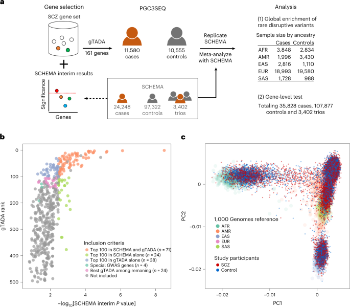
We intended to build a panel of putative SCZ risk genes from within which the majority of new discoveries from additional WES and WGS would come. To this end, we applied both traditional burden statistics and the generalized/gene set transmission and de novo association test (gTADA) to the SCHEMA data.
Traditional burden statistics
For each gene in SCHEMA, the enrichment statistics of rare variants in cases compared with controls were calculated using Fisher’s exact test separately for PTVs and damaging missense variants, then the two classes of variants were combined using meta-analysis to generate a gene-level P value. Of note, this gene-level P value is different from that in the SCHEMA publication, which used a slightly different strategy in combining PTVs and missense variants, additionally incorporated evidence from de novo mutations using trio data and included external gnomAD controls. Such analysis strategy changes in the later stage of SCHEMA have led to nontrivial changes in gene rank, which may impact the power of our panel to implicate disease genes.
gTADA
gTADA is a generalized Bayesian framework where de novo and rare variant case/control data are integrated with gene-level external information to identify risk genes for neuropsychiatric disorders33,34. We first sought to identify gene sets associated with SCZ in SCHEMA. Through curation of the literature, we identified an initial set of ~160 candidate gene sets. Next, each set was tested independently for association with SCZ in SCHEMA data using gTADA. From all of the sets tested, we identified 27 significantly enriched gene sets. We then calculated a joint enrichment Z score from the marginal Z scores and the gene set correlation matrix and kept the 25 gene sets with positive joint Z scores (Supplementary Table 2). For each of the 25 sets retained, gene-level statistics (posterior probability of being a risk gene) were then calculated. The genes were then ranked by this metric and the mean ranking across the 25 ranks was calculated.
Combining traditional burden statistics and gTADA, genes in the top 100 based on the gTADA mean ranking across the 25 ranks or the top 100 based on the minimum ranking across the 25 ranks and/or the top 100 based on the burden test were included in the panel (Fig. 1b and Supplementary Table 3; n = 139 genes; six were later removed due to the logistics of designing the sequencing panel). We next included four genes with evidence for association with SCZ in both GWASs and SCHEMA, with the criteria being: gene burden test P value < 0.05; gene with a top 200 rank in gTADA; and gene start and stop positions spanning an SNP associated with SCZ in GWAS or, if not, gene located in a GWAS locus with fewer than or equal to ten genes. Finally, an additional 24 genes were chosen for inclusion by taking the best 24 gTADA rankings of the remaining genes with a burden P value < 0.05.
Based on the observation that gene-level rare single-nucleotide variant burden statistics have been consistent across ancestries in a wide range of diseases18,19,20,21,22,23,24, our targeted panel was expected to have broad utility across ancestries, even though its construction used EUR-dominant datasets. This was further consolidated by findings from our own ancestry-stratified analysis (Fig. 2b).
Sequencing and variant calling
Ion AmpliSeq technology is an amplicon-based enrichment method for creating sequencing libraries. We used Ion AmpliSeq Designer version 6.13 to design amplicons that cover the exons of the 161 genes defined based on the Ion hg19 reference. The mean and median percentages of covered base pairs across all exons were 97.7 and 100%, respectively. Sequencing of the PGC3SEQ samples was performed on the Ion Torrent platform at Sema4 between June 2018 and April 2019. Sequencing plates were matched with respect to ancestry and case versus control composition whenever possible. The average sequencing depth across all samples was 224×. The Sema4 sequencing facility returned to the research team BAM files with flow signal and associated quality control metrics. Single-sample calling was performed using Torrent variantCaller version 5.8.0, which is specially optimized to exploit the underlying flow signal information generated by the Ion Torrent sequencing. Sites were left aligned and normalized and multiallelic sites were split into separate lines using BCFtools version 1.9 (http://samtools.github.io/bcftools/).
Genotype-level quality control
We interrogated the call set with respect to a variety of quality control metrics and implement procedures to ensure rigorous quality control standards. In the absence of well-established quality control procedures specifically for Ion Torrent data, we drew on the idea of GATK’s variant quality score recalibration technique and developed a machine-learning genotype-level filter based on 177 quality metrics and annotation profiles, including Ion Torrent sequencing metrics such as QUAL, FMT/GQ and FMT/DP, allele-related metrics such as AF, HRUN and MLLD and coverage and allele frequency from the gnomAD database version 2 (https://gnomad.broadinstitute.org). Considering that the majority of SCHEMA data with which we meta-analyzed were generated on the Illumina platform, we calibrated our Ion Torrent targeted sequencing data using a subset of the control samples (n = 1,347) with available Illumina WES data. Specifically, we used XGBoost version 1.3 (ref. 54) in Python version 3.7.3 to train the classifier in 70% of the Ion Torrent–Illumina paired data using Illumina as the ground truth. In the remaining 30% test set, the classifier achieved an area under the curve of 0.95, an accuracy of 95.3% and a false discovery rate of 4.4% for SNPs and an accuracy of 99.0% and a false discovery rate of 6.4% for indels. Applying the trained classifier to the test dataset improved the concordance between Ion Torrent and Illumina calls from 83.1 to 95.7%. We also compared our machine-learning classifier with a set of conventional hard filters and confirmed that the classifier performs unanimously better in all metrics considered (sensitivity, specificity, accuracy and false discovery rate).
Applying the machine-learning filter to the entire dataset, 83.2% of the calls were retained, and among the passed variants, 96% were SNPs and 4% were indels. Five out of 919 detected multiallelics passed the filter and were split into multiple biallelic variants. The proportion of calls that passed the filter among samples used for model training and testing (n = 1,347) and the remaining samples were similar (83.9 versus 83.1%, respectively). Likewise, the pass rate among sites that were covered by both Illumina WES capture and our sequencing panel (33.8% of the calls fell into these regions) and sites only covered by our panel were comparable (85.8 versus 81.8%), indicating that the machine-learning model generalized well to new samples and new genomic regions
Sample- and site-level quality control
To identify low-quality and outlier samples, we examined per-sample sequencing quality metrics, including the number of mapped reads, average read depth across the panel, on-target rate and uniformity rate. We also examined sample-level call set characteristics, including the call rate, inbreeding coefficient, transition-to-transversion ratio at heterozygote sites, heterozygous-to-homozygous call ratio, total number of variants, number of SNPs and indels and number of singletons. We visualized the distribution of the above quality control metrics (Supplementary Fig. 1) and identified 94 low-quality/outlier samples that met either one of the following criteria: MappedReads < 400,000; MeanDepth < 40; OnTarget < 80; Uniformity < 65; MissingCallRate > 0.3; Inbreeding_F > 0.6; Het_Hom_Ratio < 0.6; Total_SNPs < 400; and Total_Indels < 10. The number of low-quality or outlier samples was not significantly different between cases and controls (55 out of 12,045 cases were low quality or outliers and 38 out of 11,212 controls were low quality or outliers; chi-squared test, P = 0.1878). All of the quality control metrics distributed similarly between SCZ cases and controls (Supplementary Fig. 2).
When combining data from single-sample calls, a no call at a particular site in a particular sample was deemed as a homozygous reference genotype if the depth at that site in that sample was greater than ten and missing otherwise. Lastly, we applied the site-level filters to exclude variants with a missing rate of >10%.
Sample relatedness
We used the population structure-adjusted relatedness estimation methods PC-AiR and PC-Relate to estimate pairwise relatedness between samples. In addition to the quality control steps performed per previous sections, we further performed linkage disequilibrium pruning on the dataset and removed indels before relatedness estimation. Considering that the conventional kinship coefficient ranges for varying degrees of relatedness may not be appropriate when the estimates are from targeted sequencing data covering only a small fraction of the genome, we derived empirical boundaries based on the clustering of sample pairs on an identity-by-descent kinship scatterplot (Supplementary Fig. 3). The unrelated and related pairs were clearly separated into two clusters with distinct patterns (unrelated pairs: lower oval-shaped cluster; related pairs: upper left). We identified 1,096 pairs of genetic relatives and retained one sample from each pair according to the following prioritization scheme: (1) the sample has fewer genetic relatives in the entire cohort; (2) patient with SCZ; (3) the sample has available genome-wide SNP data; (4) the sample has self-reported sex information; and (5) the sample has fewer missing genotypes for variants with a minor allele frequency (MAF) of <0.1%. These measures yielded a total of 22,135 unrelated individuals for downstream analysis.
Control for population stratification
We calculated ancestry principal components for the 22,135 unrelated individuals in PLINK version 1.9 (ref. 55) using 1,392 linkage disequilibrium-pruned common SNPs (MAF > 1%) that passed all quality control steps. Cases and controls were broadly matched on population structures (Supplementary Fig. 5a,b). The first five principal components were used in later association analysis to control for population substructure, based on the observation that: (1) the first five principal components explained 75% of the cumulative variance in the genetic variation among study participants; and (2) the ability of principal components to separate ancestral genetic backgrounds dissipated after the first five principal components (Supplementary Fig. 5c).
Ancestry assignment
The genetic ancestry assignment of the PGC3SEQ participants was done by calculating principal components jointly with 1000 Genomes phase 3 participants (n = 2,501), followed by a K-nearest-neighbor classification using the top three principal components. We restricted the analysis to 1,372 linkage disequilibrium-pruned common SNPs (MAF > 1%) that were present in both the study dataset and the reference dataset (1000 Genomes). The reference data were first cleaned and quality controlled using PLINK by filtering for missingness per individual (<10%) and missingness per SNP (<10%) and then subsetted to the variant set that passed all of the quality control filters in the PGC3SEQ cohort. The cleaned reference and study datasets were harmonized, combined and pruned for linkage disequilibrium, then input into PLINK for principal component analysis with default settings.
K-nearest-neighbor classification was used for ancestry assignment of the study participants. Cross-validation determined K = 5 and the first three principal components could best classify participants into five super-populations (AFR, AMR, EAS, EUR and SAS). Applying the trained classification model, we assigned each study participant to the super-population that included the most of the participant’s five neighbors. About half of our study participants had self-reported ancestry and ethnicity data, which were broadly consistent with their genetically inferred ancestry. There was reasonable concordance between the country of origin of the sample collection and assigned ancestries (Supplementary Fig. 6).
We then ran another round of principal component analysis for each global population separately to generate ancestry-specific principal components, identified ancestry-specific outliers on the principal component plots and removed the outliers and recalculated the principal components until no obvious outlier existed. After two rounds of recalculation, two EAS and seven SAS individuals were flagged as outliers within ancestry and were not included in the analysis in which stratification by population was performed.
Variant annotation
We employed the same variation annotation workflow as was used in SCHEMA for ease of replication and comparison. Specially, annotation by LOFTEE (as implemented in the Variant Effect Predictor)56 was applied to variants that passed all quality control filters, and the analysis was restricted to the canonical transcript with the most damaging annotation. The three broad types of coding variants analyzed were: (1) PTVs, defined as any mutation that introduced a stop codon, changed the frame of the open reading frame or introduced a change at a predicted splice donor or splice acceptor site; (2) missense variants, which included any single-nucleotide variant that caused an amino acid change; and (3) synonymous variants, which resulted in no amino acid change, as a negative control. Missense variants were further partitioned into groups with increasing deleteriousness based on the MPC score annotation35. Tier 1 missense variants had an MPC score of >3, tier 2 missense variants had an MPC score of 2–3 and an MPC score of <2 indicated nondamaging missense variants. The use of MPC as the missense classifier was based on the SCHEMA results that were compared with Combined Annotation Dependent Depletion and PolyPhen; MPC most powerfully prioritized damaging missense de novo variants in ASD and developmental delay/intellectual disability trios1.
Use of SCHEMA data
SCHEMA is a large multisite collaboration aggregating, generating and analyzing high-throughput exome sequencing data of individuals with SCZ and controls to advance gene discovery. We accessed the post-quality control data of a subset of SCHEMA case–control samples with appropriate sharing permissions at the time of this work and did not reperform genotype- and sample-level filtering. Specifically, the controls from gnomAD, as included in SCHEMA, were not used in the current study due to data sharing restrictions. After excluding 216 samples detected as genetic duplicates with a PGC3SEQ sample, the available SCHEMA datasets contained 19,108 cases and 18,001 controls (Supplementary Table 4). We used the genetic ancestry label for each individual determined by the SCHEMA analysis team and, within each ancestral group, calculated population-specific principal components using linkage disequilibrium-pruned SNPs with a MAF of >1%, a call rate of >95 and a Hardy–Weinberg P value of 1 × 10⁻⁶. Using a similar procedure to that used in the PGC3SEQ data analysis, we detected and removed 24 outlier samples from the EAS group. Supplementary Fig. 7 shows the ancestral composition of the SCHEMA cohort and Supplementary Table 4 displays the number of SCHEMA cases and controls used for this study by original sample collection.
Statistical approaches for global enrichment across constrained genes
We defined rare variants as those with a minor allele count of ≤5 in the entire sample for any ancestry-combined analysis and lifted this threshold to MAF < 0.1% in ancestry-stratified analysis to preserve power. We counted the number of rare variants by annotation type observed in each participant in individual genes and added up the counts across the 80 constrained genes. The association between rare variant burden in the gene set of interest and SCZ status was tested using logistic regression with Firth’s penalized likelihood method to account for sparse data57, while adjusting for ancestry principal components and baseline rare variant burden. The first five global principal components were used in the ancestry-combined analysis and the first four principal components calculated within each ancestry were used in ancestry-stratified analysis. The baseline rare variant burden was used to control for technical and biological differences between cases and controls. To ensure a minimum correlation between the baseline burden and the burden of interest, we used the rare synonymous variant count as the baseline burden when the burden of interest was a PTV or missense variant and the rare nonsynonymous variant count as the baseline burden when the burden of interest was a synonymous variant. The significance threshold for the enrichment analysis was determined using the Bonferroni method, correcting for the five annotation classes tested (PTVs, the three missense groups and synonymous variants); that is, 0.05/5 = 0.01. P < 0.05 was used for nominal significance.
Using the available individual-level SCHEMA data, we performed global enrichment tests across the 80 constrained genes using similar approaches as in the PGC3SEQ analysis. Specifically, we used logistic regression with Firth’s correction and adjusted for ancestry principal components, sex, sequencing cohort and baseline rare variant burden. The first five global principal components were used in the ancestry-combined analysis and the first four principal components calculated within each ancestry were used in ancestry-stratified analysis.
Four of the global populations (AFR, AMR, EUR and EAS) had n > 100 in both PGC3SEQ and SCHEMA and we used inverse variance-weighted meta-analysis to combine their odds ratios in the two cohorts (sample size by population in Fig. 1a). To balance the power reduction due to sample stratification, we relaxed the definition of rare variants to include those with a MAF of <0.1% (compared with a minor allele count of ≤5 in the ancestry-combined analysis). In the full SCHEMA cohort, missense variants with MPC > 3 had a global signal on par with PTVs1; therefore, we grouped these two types of variants together in our analysis of both cohorts to further increase the power. Only PGC3SEQ contributed to the analysis of the SAS population.
Statistical approaches for gene-based tests
Gene-based tests aggregate the effects of multiple rare variants and can increase the power to detect genetic associations58. It is reasonable to assume that rare disruptive variants in a gene all have the same effect direction (variant alleles associated with higher risk) and under this scenario a burden test is appropriate. Considering the sparsity of the observed count data, we used Fisher’s exact test to compare the burden of PTVs in cases and controls and computed two-sided P values. The total disruptive burden per gene was quantified by adding up all PTVs (or synonymous variants, as a negative control) annotated to the gene. Different from SCHEMA, we did not incorporate missense variants because they were not significantly enriched globally (Fig. 2a). We did not pursue a meta-analysis of the PTV and MPC > 3 variants because the extremely low number of MPC > 3 variants prohibited a reliable estimation of their effect magnitude, which would be used as weights in a meta-analysis. Although Fisher’s exact test is not able to accommodate covariates such as ancestry principal components and baseline burden, this did not adversely affect our analysis as the Q–Q plot showed no sign of inflation in the statistics (Supplementary Fig. 10, top row).
In the gene-level analysis of SCHEMA, case–control cohorts and trio cohorts were meta-analyzed, and rare variants found in both types of cohort were not double counted. We combined gene-level P values from PGC3SEQ and SCHEMA (summary statistics obtained from the SCHEMA publication) using signed Stouffer’s method, with the sign of the Z scores being the effect direction of the PTVs and the weights of each study calculated as:
$$\frac{4}{{\frac{1}{{\# {\rm{cases}}}} + \frac{1}{{\# {\rm{controls}}}}}} + (\# {\rm{trios}}\;{\rm{in}}\;{\rm{SCHEMA}})$$
The above equation applies equal weight to the case–control data and trio data. Since only a subset of genes had de novo mutations in SCHEMA trios and the number of trios was small relative to the case–control sample size, fine-tuning weights would not meaningfully change our results. This meta-analysis totaled 35,828 SCZ cases and 107,877 controls, representing the largest SCZ sequencing dataset to date. The exome-wide significance level was determined to be 0.05/(23,321 tests performed in SCHEMA + 161 tests performed in PGC3SEQ) = 2.13 × 10⁻⁶. As expected, the meta-analysis P values deviated substantially from the null (Supplementary Fig. 10, middle left), consistent with an enrichment of risk genes in the targeted panel. Gene-level synonymous variant P values displayed the expected null distribution (Supplementary Fig. 10 (middle right) and Supplementary Table 9), assuring that the gene-level PTV results were free from technical or methodological artifacts agnostic to variant annotation.
We then combined the two SCZ cohorts with the WES datasets of two other psychiatric diseases to identify genes shared across diagnoses. The two studies from which we obtained summary statistics were: (1) the latest release of the Autism Sequencing Consortium (ASC)42 (and we further converted the gene-level q values to P values); and (2) the WES of bipolar disorder by Palmer et al.41. Meta-analysis was performed similarly as above and the same exome-wide significance threshold was also applied (2.13 × 10⁻⁶). We noted some degree of control overlap between these studies (for example, SCHEMA and ASC both included Swedish controls from the same collection). As the overlap between SCHEMA and ASC consists only a small fraction of the entire sample, our analysis (and the discovery of PCLO) should only be minimally affected. The controls overlapping between SCZ and bipolar disorder are expected to be greater per contributing cohort makeup, although we did not identify any new genes.
Reporting summary
Further information on research design is available in the Nature Portfolio Reporting Summary linked to this article.