A recent acceleration south of Cape Hatteras
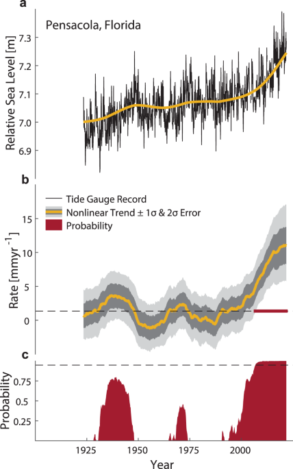
We assess nonlinear rates of MSL rise along the North American East and Gulf coasts based on 66 tide gauge records from the Permanent Service for Mean Sea Level (PSMSL) covering the period 1900–2021 (Supplementary Fig. 1). Each tide gauge record is gap-filled and corrected for linear VLM based on corrections from the recent literature7. We also consider nonlinear VLM for tide gauges along the Louisiana and Texas coastlines that are known to have been affected by fluid withdrawal16. We follow and build on an approach first introduced by ref. 16 that infers nonlinear VLM from the local differences to the tectonically relatively stable Florida Panhandle (see “Methods” for further details and validation). We use Singular Spectrum Analysis (SSA)39 to calculate nonlinear trends representative of frequencies longer than 30 years as shown, for example, by the tide-gauge record at Pensacola (Fig. 1). The rates at Pensacola, after removing VLM, have varied around an average rise of 1.4 mm yr−1 with peaks of about 3.7 mm yr−1 in the 1930s and 2.4 mm yr−1 in the 1970s. Since the early 2000s, however, MSL rates have increased to 11.1 mm yr−1 by the end of 2021. To judge whether this steep increase indeed represents a significant acceleration from its 20th century average rate, a Monte Carlo experiment is conducted. At each location, we first generate 1000 artificial time series with similar noise characteristics as tide-gauge records assuming that MSL variations are temporally correlated even at the lowest frequencies40,41 (see “Methods“). Then the observed linear trend is added to the noise and SSA-based nonlinear rates are calculated for each artificial time series. Finally, the observed rates at each time step are compared to the rates from the noise experiment representing the bounds of natural variability. If the observed rates are larger than in 95% of the cases from the artificial series, we conclude that a significant acceleration exists.
Fig. 1: Observed relative mean sea level (MSL) rise acceleration at Pensacola, Florida (PSMSL ID 246). a Monthly relative MSL record with its nonlinear trend based on Singular Spectrum Analysis (SSA) with a cutoff period of 30 years. b Rates of relative MSL rise with the 1- and 2-σ uncertainties from the noise experiment plotted around the observed rates. When the outer bound of the uncertainty envelope exceeds the linear rate (dashed line), the acceleration becomes statistically significant. The period over which this is the case is marked with a dark red line. c The corresponding probability function from the noise experiment together with the 95% threshold (dashed line) that determines the statistical significance of an acceleration. Full size image
After correcting MSL for VLM, rates along the North American East and Gulf coasts alternate around average rates of 1 and 2 mm yr−1 depending on location (Fig. 2). There are some features that appear coherently along the entire coast, such as peak rates of 3 to 5 mm yr−1 in the late 1930s and reduced rates in the 1950s. Similarly, all tide gauge records show enhanced rates of MSL rise since the late 1990s. But, in our noise experiment most of these fluctuations do not represent a significant acceleration for locations north of Cape Hatteras (except for Annapolis in the Chesapeake Bay, which we interpret as an outlier, and a couple of stations in Maine and Canada). In addition, at some locations maximum rates appear in the earlier period around 1940, such that the most recent rates are not unprecedented. South of Cape Hatteras, however, all stations exhibit their largest rates at the end of the record between 2018 and 2021. Furthermore, the rates in the south are on average 2–3 times higher than their northern counterparts and they are all significantly different from a long-term correlated random process plus linear trend since the mid-2000s (P ≥ 0.95) (Fig. 1c, Fig. 2). Such asynchronous MSL behavior across Cape Hatteras has already been noted by other studies at various time scales19,20,23,42,43,44,45,46,47,48 and periods43, and a similar separation as for the recent acceleration is also visible in the 1970s, where tide gauges experienced accelerated rates south but not north of Cape Hatteras (albeit with a smaller amplitude).
Fig. 2: Rates of mean sea level (MSL) rise along the North American East and Gulf coast since 1900. Color shadings represent the rates of (vertical land motion corrected) MSL with tide gauges arranged from Texas to Newfoundland (bottom to top) following the coastline. Rates that represent a significant acceleration from the mean rate are marked with black dots. The two dashed lines mark Cape Hatteras and the Florida Keys. Full size image
The detection of a significant acceleration extends earlier findings for the altimetry period38,45 but contrasts with refs. 18,26, who reported an acceleration hotspot between the 1970s and the end of the 2000s farther north in the Mid-Atlantic Bight and the Chesapeake Bay north of Cape Hatteras. There are several potential reasons for this. First, we use a more conservative noise model based on long-term correlations for the evaluation of the statistical significance of the acceleration, while ref. 18 only applied an autoregressive model of the order 1. Second, the approach used in ref. 18 was based on linear trend differences between two consecutive and non-overlapping 20-year periods with the most recent window spanning 1970–1989 and 1990–2009. Thus, they did not consider the high rates in the 1940s (that are also visible in their Fig. 4a), which illustrates that recent rates in this region are not unprecedented during the 20th century. Third, during the 12-year period since ref. 18 (their data ended in 2009, while data in ref. 26 ended in 2011) no further steepening of the rates has been observed. Instead, recent studies have indicated a southward shift of high MSL rates toward the South Atlantic Bight between 2010 and 2015 from satellite altimetry38,45,47. This indicates that internal variability plays an important role in the detection of acceleration “hotspots” along this coastline, a finding that will be further discussed below.
Physical causes of the acceleration south of Cape Hatteras
There are multiple possible drivers for the recent acceleration south of Cape Hatteras. The global MSL acceleration over the past decades is dominated by increased mass loss from the Greenland and Antarctic ice sheets9. However, the associated spatial GRD fingerprints are smoother and do not show an abrupt separation at Cape Hatteras7 (see also Supplementary Fig. 3). Other potential factors might be local atmospheric pressure and wind changes or contributions through river discharge anomalies49, but their signatures in coastal MSL are generally an order of magnitude smaller34,36 and show no sign of a recent acceleration (Supplementary Fig. 3). This therefore leaves only open ocean SDSL changes23 or unresolved non-linear residual VLM16 (e.g., due to uncertainties in our VLM corrections) as potential drivers of the recent acceleration.
To get a better idea whether residual VLM or SDSL changes are major drivers, we assess observations from satellite altimetry. As satellite altimetry measures MSL relative to the Earth’s center of mass, it is unaffected by any VLM. In addition, it gives a more comprehensive picture of the spatial structure of MSL variability, which may provide further indications about the processes involved. We therefore fit quadratic coefficients to both satellite altimetry and tide gauges over their overlapping period since 1993 (Fig. 3a). Positive coefficients, indicating acceleration, are visible on the continental shelf stretching from the western Gulf of Mexico along the U.S. East Coast up to Cape Hatteras. The acceleration coefficients are qualitatively consistent between satellite altimetry and tide gauges, which implies that non-linear residual VLM can be ruled out as a driver of the region-wide acceleration. We further note that the acceleration also extends offshore into the Caribbean Sea and the North Atlantic Ocean and becomes most pronounced (>1 mm yr−2) in the Subtropical Gyre region. The pattern basically mirrors the major mode of gyre-scale ocean dynamic variability (i.e., related to the expansion/contraction of the ocean) previously identified by ref. 37. This is further underpinned by a similar analysis of steric height50 of the upper 2000 m in the region (Fig. 3b). Importantly, steric height fields indicate that the pronounced acceleration is primarily induced by an expansion of the Subtropical Gyre, while the central Gulf of Mexico shows a deceleration. This, together with the knowledge that MSL varies coherently along the coast south of Cape Hatteras (Fig. 2), implies that the acceleration has likely been generated offshore23,36,46. We will return to this hypothesis below.
Fig. 3: Acceleration of mean sea level (MSL) change rates from tide gauges, satellite altimetry, and steric height over 1993–2020. a Quadratic coefficients fit to satellite altimetry and tide-gauge records (circles; after removing vertical land motion and inverted barometer contributions; see Methods). b Same as (a), but for steric height based on gridded fields derived from in-situ temperature and salinity observations from ref. 50. Full size image
SDSL in observations and historical climate model simulations
The assessment of individual MSL components above has already shown that the disagreement between observational trajectories and process-based NOAA/NASA projections in the Gulf of Mexico cannot be explained by high ice-sheet sensitivities or unresolved VLM. Rather, the acceleration seems to be consistent with an ocean-dynamic signal (Fig. 3). In a next step, we therefore aim to check how well the observations compare to the SDSL signals simulated by climate models used in the projections.
To isolate the coastal SDSL signal, we first remove an estimate of the GRD effects related to contemporary barystatic changes7 and the inverted barometer effect from each tide-gauge record (Methods). The corresponding residual rates (now primarily indicative of coastal SDSL changes) are highly coherent throughout the study area with a cluster of particularly high correlations (often exceeding 0.9) along the U.S. Southeast and Gulf coasts (Supplementary Fig. 4). This and the fact that the acceleration is geographically limited to the south leads us to do the following assessments with a median index over all stations (Methods) south of Cape Hatteras. The index is shown in Fig. 4a. The removal of the GRD and inverse barometer effects reduces the total trend at the lowest frequencies, but barely affects the decadal fluctuations in the rates including the recent acceleration. We compare this residual SDSL signal to an SDSL ensemble from historical simulations of the Coupled Model Intercomparison Project (CMIP) 551 and 652 (that have also been deployed in the recent NOAA/NASA projections) and the Community Earth System Model Large Ensemble (CESM LE)53 that employ estimates of observed (and projected) external radiative forcing (e.g., due to greenhouse gases, solar radiation, volcanic eruptions, land use, and aerosols, Fig. 4, Methods). All three historical model simulation ensembles generally mimic the multidecadal SDSL variability in observations and indicate a recent acceleration. However, the magnitude of the SDSL acceleration since the 2000s is not replicated by most models, and there is only one CMIP5 ensemble member that simulates an acceleration matching the magnitude of that seen in observations (Fig. 4a, b). This provides evidence that the disagreement between observational trajectories and model simulations in the recent NOAA/NASA report29 are indeed related to process uncertainties in the SDSL component. We also note, however, that the disagreement is not unique to the most recent period, and a similar mismatch can indeed be seen, for instance, for the peak rates in the 1970s.
Fig. 4: Nonlinear sterodynamic (SDSL) rates along the U.S. Southeast and Gulf coasts from observations and models. a Nonlinear rates of SDSL averaged from tide-gauge records south of Cape Hatteras after removing contributions from effects of Gravitation, Rotation, and Deformation (GRD) related to barystatic sea-level change, vertical land motion, and the inverted barometer effect. Also shown are the rates simulated by Climate Model Intercomparison Projection (CMIP) models 5 and 6 under historical and future forcing (RCP8.5 and SSP5-8.5, respectively) with the thick lines representing the median and shadings representing 2σ uncertainties calculated over all ensemble members. Also shown are the rates from the 38-member Community Earth System Model (CESM) Large Ensemble. b Unforced residual rates after removing the median from all CMIP5 ensemble members (thick lines). The thin lines represent rate variability estimated from 1600 (1500) phase randomized CMIP5 (CMIP6) model simulations (see Methods). The probability density distribution on the right illustrates the range of rates at the end of 2021 from those random samples. c Same as in (b), but for CMIP6. Full size image
It is important to note that while climate model simulations employ observed external forcing, each model starts with its own initial conditions54. This means that internal variability varies across ensemble members and usually does not match the phase of observed variability. Given the relatively small number of ensemble members in CMIP5 (n = 16) and CMIP6 (n = 15) it is therefore not surprising that an acceleration falls outside the range of simulations. This becomes more obvious when removing the ensemble median—an estimate of the externally forced response54—from observations and models (Fig. 4b, c). While the most recent rates are still large (exceeded only in seven (CMIP5) and two (CMIP6) percent of all cases in randomized simulations; see Methods), they are no longer significantly different to earlier highs, neither in observations nor in simulations. Rather, the observations now show an oscillating pattern with three peaks of comparable magnitude in the 1940s, 1970s and at the end of the record, indicating that the residual variability might be related to internal climate variability. We also note that the externally forced response is remarkably coherent between CMIP5, CMIP6, and CESM LE. This coherence also holds geographically, with the result that the spatial correlation clusters in the residual SDSL rates between individual sites become more distinct across Cape Hatteras after the removal of the forced response (Supplementary Fig. 4b).
Role of internal variability
As noted above, local atmospheric pressure fluctuations, coastal winds, and river discharge cannot satisfactorily explain the recent acceleration in coastal SDSL and therefore also not the mismatch between observations and the simulated forced response (Supplementary Fig. 3). Previous studies have indicated that open ocean wind stress curl variations are an important driver of seasonal to decadal MSL variations along the U.S. Southeast Coast likely through the action of Rossby waves36,44,46, albeit for shorter time scales and periods than investigated here. To test the role of wind-induced Rossby waves in the recent acceleration, we use a 1.5-layer, reduced gravity model solely forced by wind over the open ocean (see Methods). The model domain extends zonally from the west coast of Africa into the Caribbean Sea (~88°W) and solutions are calculated for each latitude between 14°N and 50°N with latitude-dependent phase speeds. We find a strong latitudinal dependence between the outputs from the reduced gravity model and unforced SDSL variations along the coast (Supplementary Fig. 5) with positive correlations at latitudes south of 20°N and north of 38°N and negative correlations at ~32°N. Maximum correlations (r > 0.7) are found with Rossby wave signals entering the Caribbean Sea near 18°N. Previous works that indicated remote open ocean signals as a driver of coastal MSL variability south of Cape Hatteras have usually interpreted the alongshore coherence (Supplementary Fig. 4) as being indicative of a signal that is communicated along the coast southward and into the Gulf of Mexico23,37. Thus, it is somewhat surprising to find maximum correlations with Rossby wave signals in the Caribbean Sea and not at latitudes close to Cape Hatteras. However, the finding is consistent with ref. 36, who also used a 1.5-layer reduced gravity model coupled to a coastal model. They demonstrated for tide gauge records at Lewes, Delaware, and Fernandina Beach, Florida, that most variance in coastal sea level can be explained when including Rossby waves from tropical regions. They suggested that the increased westward flow due to Rossby waves, after reaching the western wall, would be absorbed and diverted by the Gulf Stream system55, subsequently impacting coastal sea level northwards.
If a connection to Rossby waves in the tropics via the Gulf Stream system indeed exists, one would also expect coherence between coastal MSL along the U.S. Southeast and Gulf coasts and MSL in the Caribbean Sea. To test this, we compare the detrended coastal MSL index along the U.S. Southeast and Gulf Coast to the longest of the Caribbean tide gauge records at Magueyes Island, Puerto Rico, over the overlapping period from 1955 to 2021 (Fig. 5a). Both time series show very similar low frequency behavior with peaks in the 1970s and an acceleration over the past decade. However, the relationship is not fully in phase with maximum correlations (r~0.8 in the median index) appearing once the record at Magueyes Island leads those from the U.S. Southeast and Gulf Coasts by approximately six to eight months (Fig. 5b). As tide gauges only cover the coastal zone, we also calculate correlation maps between a central point in the Caribbean Sea (east of the Caribbean Current) and each other location elsewhere from satellite altimetry at different time lags (Supplementary Fig. 6). At a zero lag, large correlations are confined around the Caribbean Islands with a narrow strip of high positive correlations stretching into the Gulf Stream path. After six to eight months, however, correlations in the Gulf Stream path become larger, extend over larger parts of the Subtropical Gyre, and reach into the coastal zones in the Gulf of Mexico. These results support the idea of an advective transfer of density signals from the Caribbean Sea via the larger Gulf Stream system into the Gulf of Mexico and the coastal zones south of Cape Hatteras. This is further supported by recent sensitivity experiments in the adjoint model of the Estimating Circulation and Climate of the Ocean system56 that pointed to a strong physical linkage between MSL in Charleston, South Carolina, and wind stress forcing (as well as heat and freshwater fluxes) over the Caribbean Sea (maximizing when the latter leads by four to eight months). In line with that, ref. 57 showed that flows through the Gulf of Mexico and the Florida Straits are driven by wind stress curl variations over the tropical North Atlantic. More dedicated ocean model sensitivity experiments will be required to further clarify the impact of Rossby waves onto the Gulf Stream system, the mechanisms by which these signals are transferred into the coastal zones, and what time lags are involved. Those are, however, beyond the scope of this study.
Fig. 5: Comparison between mean sea level (MSL) variability along the U.S. Southeast and Gulf coasts and the Caribbean Sea. a Individual linearly detrended tide gauge records over their overlapping period from 1955 to 2021. All time series have been smoothed with a moving average filter of 48 months. b Lead-lag correlation analysis; the left side indicates correlations when the Caribbean Sea leads, while the right side indicates lagged correlations. Full size image
To estimate the integrated gyre-scale effect of wind-forced Rossby waves on coastal sea level south of Cape Hatteras, we isolate the leading modes of variability from the reduced gravity model using principal component analysis (Supplementary Fig. 7, see Methods). The combined signal captures major decadal events such as the highs in the 1940s, 1970s and the large increase over the past decades and its amplitude is dominated by variations originating from the tropics, particularly southeast of the Gulf of Mexico inflow region (Supplementary Fig. 7). Again, this suggests a dominance of advective processes from the south leading to an expansion of the larger Subtropical Gyre region (Fig. 3b). Farther north, where the Gulf Stream is detached from the coast, coastal MSL has rather been linked to density anomalies in the Subpolar Gyre (amongst other factor such as local coastal alongshore wind)22,23 giving a plausible explanation for why the recent acceleration has been limited to the south. When we combine the resulting Rossby wave signals with other internal forcing factors, notably river discharge49 and coastal winds20 (Fig. 6), we find correlations of r = 0.8 with unforced SDSL variability. This suggests that a major fraction of the residual SDSL variability is indeed internally forced and that changes in large-scale wind stress curl over the tropical Atlantic have contributed significantly to the recent acceleration as well as earlier peaks in rates of MSL rise (Fig. 6a). Other factors, such as astronomical cycles, may have also contributed to the recent acceleration as well, but their amplitude is very small compared to the processes discussed here22.