Recruitment and participants
Participants were recruited via on-campus advertisements, email, and the online data collection platform agestudy.nl. A Dutch subject registry (hersenonderzoek.nl) was used to approach participants to join agestudy.nl53. This study pooled data across completed21,28,54 and ongoing data collections involving smartphone behavioral recordings in self-reported healthy participants (data collection frozen on the 2nd of June 2022). The inclusion criteria were: (a) users with personal (unshared) smartphones with the Android operating system, (b) self-reported healthy individuals, (c) with no neurological or mental health diagnosis at the time of the recruitment, and (d) a minimum of 90 consecutive days of smartphone data. This resulted in 412 participants (age: min. 16 years, max. 84 years, median 59 years), and 403 reported their gender (64% females). All participants provided informed consent (using a checkbox on the study platform for subjects who were only engaged online or using written signatures for subjects visiting the laboratory) and the data collection was approved by the Psychology Research Ethics Committee at the Institute of Psychology at Leiden University.
Smartphone behavioral recording and the joint-interval distribution
A background app (TapCounter, QuantActions AG, Zürich) was used to record the timestamp of all smartphone touchscreen interaction events55. The timestamp of the event onset – say towards a swipe or a tap – was recorded in UTC milliseconds. The data was collected using a unique participant identifier linking to the self-reported age, and gender. The background app also logged the label of the App in use but this information was not used here. Apart from the touchscreen events, the App also recorded the screen “on” and “off” events which were used to define within-session interactions. The taps.ai (QuantActions AG, Zürich) was used to monitor the data collection. The platform alerted the investigators if the participants failed to provide the device permissions necessary to collect the timestamps (at the app installation stage during the study registration) and if no data was streamed to the servers for > 24 hours during the collection from a particular device. Users were contacted to resolve any data discontinuity (or the users confirmed the absence of use or connectivity). Based on these interactions (not annotated) a common reason for data discontinuity (according to the attending researchers) was the app failing to restart after the phone was shut down, and this was simply resolved by manually launching the app. The app-related data discontinuities were most prevalent in Huawei phones (33 devices, and on average 17% of the days missed data), and the full list of the extent of missed data per model and Android version is in Supplementary Table 1 and Supplementary Table 2 respectively.
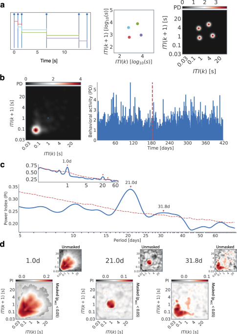
Within the session (between a screen “on” event and a screen “off” event) intertouch intervals (ITIs) were used to estimate joint-interval distributions. The intervals were accumulated in consecutive 1-hour bins. For each hourly bin, the duration of an interval with index k was related to that of the subsequent interval k + 1, thus creating a two-dimensional map of events. We consider each subsequent pair of events as being sampled from a joint-probability distribution \(P\left( {k,k + 1} \right)\), and this estimated the continuous two-dimensional joint probability distribution over the log 10 transformed space using kernel density estimation with a Gaussian kernel and a bandwidth of 0.1 (KernelDensity, sklearn, python). We limited our range of estimation between 101.5 ms (~30 ms) to 105 ms (~2 min), with the upper bound corresponding to the 99th percentile of all observed inter-events. We discretize the space in 50 steps in each dimension thus obtaining a behavioral space of 50 × 50 x \(D\), where \(D\) is the recording duration in hours.
Wavelet transformation and block-bootstrap
The continuous wavelet transform (cwt, MATLAB, MathWorks, Natick) of the time-series of each two-dimensional bin of the JID was based on a filter bank (cwtfilterbank, MATLAB) with the following parameters: sampling period of 1 hour, voices per octave of 40, and period limits from 2 hours to 80 days. The cone of influence was removed before estimating the periodogram power (P) at a given period (t), where the matrix S t contained the wavelet transformed spectral values [Eq. (1)]:
$$P_t = \sqrt {\overline {|S_t|} }$$ (1)
The time series was block-bootstrapped with a 24-hour window, and the wavelet transform was estimated for each bootstrap (number of targeted bootstraps 1000)24. The bootstrap computations were performed on a high-performance computing cluster (ALICE, Leiden University). The computations failed in 11 of the participants, resulting in an N of 401. The mean of the bootstrapped values was used to capture the aperiodic component of the periodogram, and it was subtracted from the real to obtain the adjusted periodogram (power index).
The significant periodogram values were isolated based on a two-tailed α = 0.05 based on the bootstrapped periodogram. This was subsequently corrected for multiple comparisons using clustering (LIMO EEG39) across the JID feature space and period such that a cluster contained significant values in 5 neighboring bins. Briefly, the cluster sizes were accumulated for each boot against the rest of the boots, and the maximum cluster size was noted for each iteration. Only those clusters based on real data which were >97.5th percentile of the iterated set of maximum clusters were considered significant.
Non-negative matrix factorization
For each individual the spectral computations using wavelet transform resulted in a tensor of the dimension of the JID (50 × 50 x T), where T is the number of periods in the periodogram and is a function of the recording length (in the population min. T was 335, max. was 396). The bootstrap-derived aperiodic component was subtracted from this tensor. The tensor was then sliced along the periods dimension to select only the periods between \(P_{min}\) (with index \(i_{P_{min}}\)in the periods list) and \(P_{max}\) (with index \(i_{P_{max}}\)in the period list) reshaped into a matrix of sizes \(T^\prime \times 2500\) where \(T^\prime = i_{P_{max}} - i_{P_{min}}\). The matrix was then globally shifted up by subtracting the global minimum rendering it non-negative.
The non-negative matrix factorization (mexTrainDL, spams package for MATLAB, Inria) yielded two matrices: a meta-rhythms matrix \(W \in {\Bbb R}^{T^\prime \times R}\)and a meta-behavior matrix \(H \in {\Bbb R}^{R \times 2500}\) where R is the optimal factorization rank. The optimal rank for the factorization was estimated using cross-validation. For the cross-validation, we repeated the factorization for ranks from 3 to 15. We randomly selected 10% of the entries from the matrix to be masked and used as a test set. The factorization was done on the matrix with masked values. After the factorization, the test error was obtained by evaluating the reconstruction error of the 10% of entries that were left out (test set). We repeated this process 100 times for each rank. The optimal rank was defined as the rank with the minimum mean test error across the 100 repetitions. The optimal rank varied from person to person with a minimum rank of 3 and a maximum rank of 14. The factorization was performed for all the subjects (N = 401) with \(P_{min} = 2.2\) days and \(P_{max} = 27.7\) days \(i_{P_{min}} = 180\), \(i_{P_{max}} = 336\), thus \(T^\prime = 147\). And separate factorization was performed for subjects with at least 180 days of data (N = 218) with \(P_{min} = 2.2\) days and \(P_{max} = 70.5\) days, \(i_{P_{min}} = 190\), \(i_{P_{max}} = 360\), thus \(T^\prime = 201\). Note, although the seven individuals who did not report their gender were included in the factorization they were omitted from the plots.
While non-negative matrix factorization is a powerful dimensionality reduction method, it is known to be susceptible to its initial conditions and can lead to different factorizations if repeated with the same input matrix56. To mitigate this issue, for each individual we repeated the following procedure to pick the most reproducible (as defined below) decomposition. We coin this stable and reproducible, starNNMF: Given the best rank calculated with the procedure described above, we repeated the decomposition 1000 times with different initial conditions. We then calculated the pairwise correlation coefficient for each pair of decompositions (using the meta-rhythms matrix) by calculating the cross-correlation matrix across components and picking the highest correlation across the components (meta-rhythms). For each decomposition, we then computed the median of the pairwise cross-correlation with all other decompositions and picked as the final decomposition the one with the highest median correlation across the 1000 repetitions.
We clustered the meta-rhythms accumulated across the population by using a one-dimensional continuous wavelet transform (mdwtcluster, MATLAB). This was inspired by57. The one-dimensional CWT clustering uses all the coefficients from a Daubechies 4 wavelet. We first z-scored each meta-rhythm. Then we estimated the optimal number of clusters by using the silhouette method (evalclusters, MATLAB). Finally, we operationalized the clustering with the obtained best number of clusters. The best number of clusters emerged to be 5 for the analysis up to 27.7 days and 7 for the analysis up to 70.5 days. Note, that since we considered each meta-rhythm independently and each subject had a different number of meta-rhythms, each individual could contribute with zero to multiple meta-rhythms to a given cluster.
Phase coherence analysis
We selected 175 subjects with at least 180 days of overlapping recordings. We then extracted a range of periods for each cluster corresponding to the periods surrounding the peak of the mean meta-rhythm across the cluster. More specifically, for each cluster, we first calculated the mean across the cluster. The location of the peak of the mean was thus identified as the reference period for that meta-rhythm cluster. To get the ranges for each peak (min/max range), we first estimated the 95th percentile of the mean of the cluster, and then we created a binary vector indicating where the values of the mean cluster were > 95th percentile, the min. range is the period corresponding to the minimum index that has a 1 in the above binary vector, while the max. range is the period corresponding to the maximum index that has a 1 in the above binary vector.
For each subject and each period range, we selected the JID two-dimensional bin with the maximum power index located in the largest statistical cluster (largest in terms of the overall number of significant pixels for a select period). For each pair of subjects (thus selected JID) we extracted the probability density of that pixel from hourly JIDs. We calculated the CWT spectral coherence based on the same filterbank and wavelet described above (wcoherence, MATLAB). Over the spectral coherence spectrum, we selected the period range of interest and estimated the average coherence. This was repeated for all possible pairs and at every discovered multiday rhythm. The coherence values above 95th percentile (corresponding to one-tail α = 0.05) of 24-hours block bootstrapped data (~1000 bootstraps as mentioned above) were considered significant.
Reporting summary
Further information on research design is available in the Nature Research Reporting Summary linked to this article.