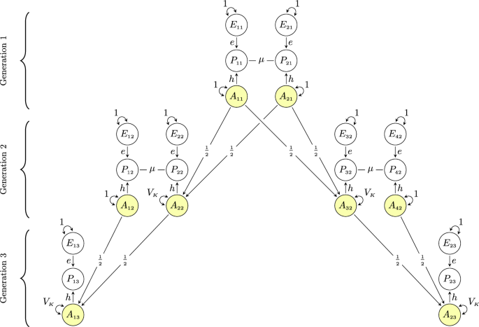
Figure 1 shows a theoretical model of similarity in extended families in the presence of assortative mating at intergenerational equilibrium. The model includes eight individuals (\(i\)) in three generations (\(t\)): two partners in the first generation, their two children in the second generation (who are each other’s full sibling) along with their respective partners, and two children in the third generation (who are each other’s first cousin). The phenotype that is assorted on is denoted with \({P}_{{it}}\), whereas trait-associated additive genetic factors and unique environmental factors are denoted with \({A}_{{it}}\) and \({E}_{{it}}\), respectively. The genotypic correlation between any two individuals is the sum of all valid chains of paths between their respective additive genetic factors and the value of a single chain is the product of its path coefficients33,34. Valid chains always begin by tracing backward (←) in relation to the direction of arrows, incorporating exactly one double-headed arrow (↔), after which tracing continues in a forward direction (→). Because the variables in Fig. 1 have unit variances, all valid chains connecting a variable to itself will sum to 1, allowing us to immediately trace in a forward direction (i.e., change direction at once). Copaths (—), which are arrowless paths representing associations arising from assortment35, link together valid chains per the rules above, forming longer, valid chains. For a more detailed description of path tracing rules involving copaths, see Balbona et al.36 or Keller et al.37 Path diagrams with relaxed assumptions (e.g., gene-environment correlations) are presented and discussed in Supplementary Notes 1–3, whereas simulations validating our theoretical expectations are presented in Supplementary Notes 4 and 5.
Fig. 1: Path diagram of similarity in extended families under assortative mating. Path diagram for a model of genetic similarity in extended families under phenotypic assortative mating at intergenerational equilibrium (i.e., equal variance across generations). The partner correlation attributable to assortment is denoted by \(\mu\), the recombination variance is denoted by \({V}_{K}\), and \(h\) and \(e\) denote the effect of additive genetic (\({A}_{{it}}\)) and environmental factors (\({E}_{{it}}\)), respectively, on the phenotype (\({P}_{{it}}\)) of individual \(i\) in generation \(t\). All variables have unit variance, meaning \(e=\sqrt{1-{h}^{2}}\) and \({V}_{K}=\frac{1-\mu {h}^{2}}{2}\). See the Supplementary Notes 1–3 for path diagrams with relaxed assumptions. Full size image
Expected genotypic correlations in the nuclear family
In Fig. 1, there is only one valid chain between partners’ additive genetic factors (e.g., \({A}_{11}\) ↔ \({A}_{21}\)): \(h\times \mu \times h\). The genotypic correlation between partners (denoted \({\rho }_{g}\)) is thus the phenotypic correlation attributable to assortative mating, \(\mu\), weighted by the trait’s heritability, \({h}^{2}\):
$${\rho }_{g}=\mu {h}^{2}$$ (1)
Similarly, we can trace the valid chains between the additive genetic factors of a parent and their offspring (e.g., \({A}_{11}\) ↔ \({A}_{22}\)). There are two valid chains: one directly from parental genetic factors to offspring genetic factors, \(\frac{1}{2}\), and one through the other parent via the assorted phenotype: \(h\times \mu \times h\times \frac{1}{2}\). The genotypic correlation between parent and offspring is therefore \(\frac{1}{2}+\frac{h\mu h}{2}\). With no assortative mating (\(\mu=0\)), this reduces to \(\frac{1}{2}\). For siblings (\({A}_{22}\) ↔ \({A}_{32}\)), there are four valid chains: \(\frac{1}{4}+\frac{1}{4}+\frac{h\mu h}{4}+\frac{h\mu h}{4}\), which can be rearranged so that it equals the genotypic parent-offspring correlation. Because they are equal, we can define a common denotation (\({r}_{{g}_{1}}\)) for first-degree relatives. We can also substitute \(h\times \mu \times h\) with \({\rho }_{g}\) giving us:
$${r}_{{g}_{1}}=\frac{1+{\rho }_{g}}{2}$$ (2)
In other words, the genotypic correlation between first-degree relatives, \({r}_{{g}_{1}},\) is increased by half the genotypic correlation between partners at equilibrium. (Note that the phenotypic correlation will not be the same for siblings and parent-offspring despite the same genotypic correlation3). An advantage of using path analysis is how easy path diagrams are to expand. In the Supplementary Information, we detail how relaxing the assumption of equilibrium (Note 2) and including polygenic indices (Note 3) changes the correlations. During disequilibrium, the genotypic correlation between partners will still conform to Eq. (1), but the correlation between relatives will be less than what Eq. (2) would predict. For polygenic index correlations, one must include a term representing the imperfect correlation between the polygenic index and the true genetic factor. The polygenic index correlation between partners should therefore be:
$${\rho }_{{pgi}}=\mu {h}^{2}{s}^{2}$$ (3)
where \({s}^{2}\) is the shared variance between the polygenic index and the true additive genetic factor (i.e., the genetic signal19). Assortative mating will induce covariance between different loci (i.e., linkage disequilibrium), which is included in the genetic signal. This means that \(s\) may be larger than the correlation between the true direct effects and the polygenic index weights, and as such do not represent the accuracy of the polygenic index weights (see Supplementary Notes 3, 4.4, and 5.6). If the genetic signal is low, the polygenic index correlation between partners will be biased towards zero compared to the true genotypic correlation19. For first-degree relatives, the equation becomes similarly altered, but because the error terms in the polygenic indices are correlated between relatives, the polygenic index correlation will be biased towards the coefficient of relatedness rather than zero:
$${{r}_{{pgi}}}_{1}=\frac{1+{\rho }_{{pgi}}}{2}$$ (4)
Expected genotypic correlations in the extended family
The model in Fig. 1 has two properties that allow a general algorithm to find the expected genotypic correlation between any two members in extended families. First, all the chains that connect the genotypes of first-degree relatives can readily be continued without breaking path tracing rules. Second, all chains between the genotypes of any two related individuals are mediated sequentially through the genotypes of first-degree relatives. The genotypic correlation between \({k}^{{th}}\)-degree relatives, denoted \({r}_{{g}_{k}}\), can thus be attained by raising the genotypic correlation between first-degree relatives to the degree of relatedness:
$${r}_{{g}_{k}}={\left(\frac{1+{\rho }_{g}}{2}\right)}^{k}$$ (5)
For example, the expected genotypic correlation between third-degree relatives like first cousins is \({(\frac{1+{\rho }_{g}}{2})}^{3}\), which can be verified by manually tracing all valid chains between \({A}_{13}\) and \({A}_{23}\) in Fig. 1. The genotypic correlation between non-blood relatives like in-laws, which will be non-zero under assortative mating, can be attained by linking together chains of \({r}_{{g}_{k}}\) and \({\rho }_{g}\) (for example, \({Corr}\left({A}_{12},{A}_{42}\right)={r}_{{g}_{1}}{\rho }_{g}^{2}\)). As for polygenic index correlations, they can be approximated by replacing \({\rho }_{g}\) with \({\rho }_{{pgi}}\) in Eq. (5), although depending on the genetic signal, the true correlation between polygenic indices may be slightly higher (see Supplementary Note 3).
Figure 2 shows how assortative mating changes genotypic correlations between relatives at equilibrium. In Panels A and B, it is evident that assortative mating has a much larger effect on first cousins than full siblings. For example, for a trait where \(\mu=.50\) and \({h}^{2}=50\%\) (meaning \({\rho }_{g}=.25\)), siblings (Panel A) will have a correlation of \({r}_{{g}_{1}}=.625\) whereas cousins (Panel B) will have a correlation of \({r}_{{g}_{3}}=.244\), reflecting increases of 25% and 95%, respectively, compared to random mating. Panel C shows how this pattern extends to more distant relatives, with the genotypic correlation between second cousins 3.5 times higher than normal if \({\rho }_{g}=.25\) (\({r}_{{g}_{5}}=.095\) vs. \(.031\)). The larger relative increase is not merely because the correlations are smaller to begin with: Panel D shows that the largest absolute increase typically occurs in second-degree relatives like uncles/aunts and nephews/nieces.
Fig. 2: Assortative mating’s effect on genotypic correlations between various relatives. A, B The expected genotypic correlation (\({r}_{g}\)) at equilibrium between full siblings (i.e., first-degree relatives) and first cousins (i.e., third-degree relatives) under different combinations of assortment strengths (\(\mu\)) and heritabilities (\({h}^{2}\)). C, D The relative and absolute increase in genotypic correlation at equilibrium for various relatives and genotypic correlations between partners (\({p}_{g}\)). Full size image
The relatively greater increase in correlation between cousins is because third-degree relatives are affected by three assortment processes: Mother-father, uncle-aunt, and grandfather-grandmother partnerships are all correlated under assortative mating and contribute to the increased correlation (Fig. 1). For each additional degree of relatedness, there is an additional assortment process opening pathways for relatives to correlate. This pattern extends to unrelated individuals like siblings-in-laws, who would have a genotypic correlation of \({\rho }_{g}{r}_{{g}_{1}}=.157\) if \({\rho }_{g}=.25\). It is evident that assortative mating has a relatively larger impact on the genotypic correlation between distant relatives compared to close relatives, and that heritable traits subject to strong assortment can produce significant genotypic correlations between family members who would otherwise be virtually uncorrelated.
Gene-environment correlations, shared environment, and dominance effects
One limitation with most earlier work, such as Fisher1, is that they assume a simplistic model where genetic similarity is the only cause of familial resemblance. In Supplementary Note 1, we detail how genetic similarity between relatives are affected by dominance effects, shared environmental effects, and various forms of environmental transmission. If genetic and environmental transmission occur simultaneously, assortative mating will induce (and greatly increase) correlations between genetic and environmental factors. Such gene-environment correlations will, in this context, mimic higher heritability, leading to higher genotypic correlations between partners and thereby exacerbated genetic consequences of assortative mating. However, the relationship between the genotypic correlation between partners and the genotypic correlation between first-degree relatives will stay the same, meaning Eq. (2) and Eq. (4) can be used without making assumptions about gene-environment correlations or other sources of familial resemblance.
This is not the case for distant relatives. If there are substantial shared environmental effects, gene-environment correlations, or other sources of familial resemblance, the properties of Fig. 1 that allow the general algorithm in Eq. (5) are no longer present. This is because non-genetic causes of familial resemblance result in pathways between distant relatives that bypass the genotypes of intermediate relatives, thus increasing the true genotypic correlation to beyond what Eq. (5) would predict. Equation (5) still serves as a rough approximation, although any statistical model that relies on it could be biased if such extra pathways exist.
Empirical polygenic index correlations between partners and relatives
Figure 3 shows polygenic index correlations between family members for a range of traits. Nine out of sixteen traits were significantly correlated between partners (Panel A), including height (0.07), body mass index (0.04), intelligence (0.04), and educational attainment (0.14). When educational attainment was split into cognitive and non-cognitive factors (GWAS-by-subtraction38), we find roughly equal partner correlations for both components. Psychiatric traits like ADHD, depression, cross-psychiatric disorder, and bipolar disorder exhibited no significant correlations between partners. Keep in mind that the correlations will be biased downwards to the extent the genetic signal is poor (ref. Equation (3)).
Fig. 3: Correlations between family members. Polygenic index correlations (with 95% CIs) for various traits between various family members: (A) partners (N = 47,135), (B) full siblings (N = 22,575), (C) parent-offspring (N = 117,041), and (D) first cousins (N = 28,330). The vertical dashed lines are the expected correlation under random mating (i.e., the coefficient of relatedness), and the black crosses are the expected correlation at equilibrium given Eq. (5). Abbreviations: EA educational attainment, BMI body mass index, IQ intelligence, ADHD attention-deficit hyperactivity disorder. Correlations are also reported in Supplementary Table 17. Full size image
Panels B, C, and D show polygenic index correlations between full siblings, parents and offspring, and first cousins, respectively (see Supplementary Fig. 29 for other family members). The vertical dashed lines are the expected correlations under random mating and the black crosses are the expected correlations at equilibrium given the partner correlation and Eq. (5). All traits with significant correlations between partners had significantly higher parent-offspring correlations than would be expected under random mating, and we observed similar patterns for other relatives. For example, the polygenic index correlation for educational attainment was 0.56 (instead of 0.50) between full siblings and 0.20 (instead of 0.125) between first cousins.
Testing intergenerational equilibrium
We fitted structural equation models using mother-father-child trios to see if a model constrained to equal variance across generations (i.e., equilibrium) resulted in significantly worse fit (see Supplementary Note 6). Six out of nine traits were significantly different from equilibrium. We also investigated two consequences of disequilibrium, namely greater variance in the offspring generation (Fig. 4A) and smaller-than-expected parent-offspring correlations (Fig. 4B). During disequilibrium, the ratio of offspring polygenic index variance to parental polygenic index variance should be positive: \({Q}_{{pgi}}=\frac{{Offspring\; Variance}}{{Parental\; Variance}}\) (see Supplementary Notes 2.1 and 3.3). However, this ratio is quite sensitive to the genetic signal of the polygenic index, and therefore provides limited information about the history of assortative mating beyond demonstrating disequilibrium. An alternative measure that is less sensitive to the genetic signal is the observed increase in polygenic index correlation as a percentage of the expected increase19: \({U}_{{pgi}}=\frac{{Observed\; Increase}}{{Expected\; Increase}}\) (see Supplementary Notes 2.3 and 3.4). This provides a measure of how close the trait is to equilibrium. By comparing \({U}_{{pgi}}\) to reference values under various heritabilities and assortment strengths, it is possible to infer the equivalent number of generations of stable assortative mating if starting from a random mating population. If the parental generation was the first generation to mate assortatively, we would expect \({U}_{{pgi}}\,\approx\, 70\%\), while we would expect \({U}_{{pgi}}=100\%\) if the trait was in equilibrium.
Fig. 4: Tests of intergenerational equilibrium. Parameter estimates (with 95% likelihood-based CIs) from structural equation models using mother-father-child trios (N = 87,896 families, 35,025 of which were complete). A Ratio of offspring polygenic index variance to parental polygenic index variance (\({Q}_{{pgi}}\), see Supplementary Note 2.1). A value above 1 would indicate that the variance is greater in the offspring generation compared to the parental generation, as expected during disequilibrium. B Observed increase in parent-offspring correlation compared to expected increase at equilibrium (\({U}_{{pgi}}\), see Supplementary Note 2.3). A value of about 70% would indicate that the parent generation was the first generation to assort on this trait, whereas 100% would indicate that the trait is in intergenerational equilibrium. Only traits with significant correlations between partners are shown. Shape corresponds to trait types in Fig. 3, where circles are anthropometric traits and squares are psychosocial traits. Abbreviations: EA educational attainment, BMI body mass index, IQ intelligence. Full size image
Height did not deviate from equilibrium: There was no significant difference between the parental and offspring variance nor between the observed and expected correlations. The results for drinking and smoking behavior were also consistent with equilibrium, although the observed partner correlation was too small to make this test informative. Body mass index and other psychosocial traits, on the other hand, did deviate from equilibrium: For example, the polygenic index variance for educational attainment was 2.46% greater in the offspring generation compared to the parental generation. The true genetic variance ratio is likely much larger: For example, if the polygenic index captures one third of the true genetic factor (\({s}^{2}=1/3\)), then the true variance increase would be approximately 7.4% (see Supplementary Note 3.3). The parent-offspring polygenic index correlation was also slightly but significantly lower than expected at equilibrium (\({U}_{{pgi}}=90\%\), 95% CIs: \(87{-}93\%\)). When we compared this to calculations of what the observed increase would have been after successive generations of assortative mating, we found that \({U}_{{pgi}}=90\%\) is equivalent to approximately three generations of stable assortment (see Supplementary Note 2.3). Results were similar for other psychosocial traits, albeit with somewhat shorter implied histories. Body mass index, on the other hand, had a parent-offspring polygenic index correlation that would imply that the parent generation was the first to mate assortatively (\({U}_{{pgi}}=71\%\), 95% CIs: \(60{-}81\%\)). This would also explain why the sibling correlation – many of whom are in the parent generation – was not higher than expected under random mating.