Analysis approach
Conducting a detailed analysis of aeroplane crashes in the ocean is challenging due to the limited number of occurrences. Despite the scarcity of data, the unique and energetic nature of such events, coupled with a relatively low frequency of occurrence of signals with similar characteristics, presents an opportunity for insightful analysis. For instance, the highest relevant signal frequency observed in the analysis was four signals in 10 min, in Fig. 9a, highlighting a constrained set of possibilities. Considering the 10-min window and allowing for a 2\(^{\circ }\) uncertainty in the bearing (which is much larger than the maximum deviation), the probability of a signal occurring by chance, unrelated to the event, is less than 3%. This high level of confidence (97%) in the signal’s relevance to the event arises from the limited occurrences and distinctive characteristics of the signals. Even with a broader 20-min window, featuring eight signals and a more lenient 5\(^{\circ }\) bearing uncertainty, the probability of the signal being unrelated to the event remains below 12%. However, it is acknowledged that the disadvantage of this approach emerges when the impact location is unknown, leading to an increased degree in bearing uncertainty.
It is worth noting that in the calculation of the acoustic speed, although average speeds can be calculated with precision, the methodology employed here takes a broader perspective. Rather than focusing solely on accuracy, the approach involves exploring the entire spectrum of possibilities, even if it means incorporating seemingly irrelevant signals. This ensures that no potential signal of interest is inadvertently overlooked. Therefore, prior to diving into the sufficient conditions to correlate the signal with the incident, the necessary conditions are first examined. This approach is chosen due to the limited number of signals that meet the necessary conditions as described above.
Signal processing and bearing calculation
Signals from past aircraft crashes were presented around the middle of a 10 min time window, to allow visual comparison. Spectrograms indicate the frequency band of noise as opposed to frequency bands from signals. Most processed signals show a significant amount of noise in the 0–4 Hz band. Noting that the broadband frequency content is typical for the propagation of acoustic-gravity waves15 that can travel far distances from the event location, a high pass Butterworth IIR filter was used (in addition to the CTBTO high pass filter) below 5 Hz. Moreover, a 2–40 [Hz] band-pass filter was applied in general. Filtering noise, enhancing the signal appearance and stabilising the time-waveform can be crucial for identifying the bearing of the signal of interest, in particular when the source is an impulse that generates short signals of a few seconds length.
Each hydrophone station has three hydrophones configured in a triangular shape spaced by around 2 km. Exact locations of all hydrophones can be obtained from the CTBTO. In information theory, entropy serves as a measure quantifying the amount of information encapsulated within a signal. Let \(P(x)\) denote the probability distribution function of the discrete-time signal \(x\), then the entropy is defined as
$$\begin{aligned} H(x) = - \sum P(x) \cdot \log _2 P(x). \end{aligned}$$ (1)
Additionally, log energy entropy16, represented as \(H_L\), is defined as:
$$\begin{aligned} H_L = - \sum P(x) \cdot \log _2 P(x). \end{aligned}$$ (2)
Windowed entropy calculations can be employed to identify transient signals against a noisy background. This is predicated on the assumption that the randomness measure of the signal will exhibit changes when the nature of the signal undergoes alterations. Entropy values have been computed across a window size of a few seconds and a step size of 0.5 s. As depicted in Figs. 11 and 12, peaks in the entropy trace emerge where transient signals are detected. A threshold of \(2.3 \times 10^4\) has been established; all peaks within a 2-second window across all signals are considered for subsequent bearing calculations. Note that the frequencies of the signal of interest, are within a frequency band, say below 20 Hz, which is order of magnitude lower than the sampling rate of the hydrophones (250 Hz). Thus related errors are expected to be small17.
Following the isolation of signals of interest, bearing determination is carried out using time-of-arrival-based triangulation. The time of arrival is estimated by identifying the maximum of the cross-correlation function across channel pairs, enabling the derivation of pairwise time of arrival differences \(t_i - t_j = \Delta _{ij}\). Geometric parameters for the array are derived from latitude and longitude position data corresponding to the hydrophones. Assuming a constant arrival velocity v an expression of the geometric parameters is given by13
$$\begin{aligned} \theta = \cot ^{-1}\left[ \frac{L_{23}}{L_{12}\sin (\alpha +\beta )}\left( \frac{\Delta _{21}}{\Delta _{32}}-\frac{L_{12}}{L_{23}}\cos (\alpha +\beta )\right) \right] \end{aligned}$$ (3)
with parameters defined in Fig. 13, with no loss of generality. Using a 99.5% confidence interval, the bearing calculations are considered to be accurate to \(\pm 0.4^{\circ }\) (see Ref.13 for more details).
Figure 11 illustrates how high noise to signal ratio can prevent calculating the bearing of the signal of interest. In particular, the figure concerns bearing calculations of signals from airgun shots on Fig. S1c. Clearly, the airgun bearing of \(210^{\circ }\) (highlighted in magenta) dominates the picture, which prevents calculating the bearing of the signal of interest at 19:05 UTC. On the other hand, Fig. 12 provides a successful capture of the bearing of the signal of interest \(269^{\circ }\) (highlighted in magenta) 19:41 UTC.
Figure 11 Bearing calculations of signals on Fig. S1c. From top to bottom: recordings from three channels at station H08S between 19:00 and 19:10 UTC on March 7th 2014. Windowed entropy shows peaks (black triangles) where a transient signal is found. Each peak defines an event, for which bearing is calculated from differences in arrival times in the bearing subplot. The map demonstrates the dominating bearing from airgun signals, \(210^{\circ }\) (highlighted in magenta), which prevent calculating the bearing of the signal of interest at 19:05 UTC. Full size image
Figure 12 Bearing calculations of signals on Fig. S1e. From top to bottom: recordings from three channels at station H11S between 19:41 and 19:51 UTC on March 7th 2014. Windowed entropy shows peaks (black triangles) where a transient signal is found. Each peak defines an event, for which bearing is calculated from differences in arrival times in the bearing subplot. The map illustrates the direction of the calculated bearings. The bearing of the signal of interest at 19:46 UTC is successfully calculated as \(269^{\circ }\) (highlighted in magenta). Full size image
Figure 13 Geometry of the three hydrophones array and bearing calculation. Credit: Fig. 9 of Ref.13. Full size image
Possible impact location near the 7th Arc
A comprehensive list of signals potentially recorded near the 7th arc shortly after the last handshake are given in Table 1. The only major signal has a bearing of \(306.18^{\circ }\), and it is recorded at 00:54 UTC. In that direction the distance of the 7th arc from H01W is \(R_7=1586\) km. For an acoustic signal travelling with a speed of \(c=1500 \,{\pm \,70}\) m/s, the required time to travel from the 7th arc to the H01W is \(17.45\pm 0.65\) min. The time difference between the 7th arc and the time the signal was recorded is 34.5 min. Thus, if the signal is associated with the aircraft crash then there is an extra time of \(\Delta t = 17.02\pm 0.65\) min. Therefore, if the airplane was travelling at an average velocity \(\bar{v}\) (defined positive in the direction of the bearing), it will travel away from the 7th arc a distance \(\Delta \bar{r}\) during time \(\Delta T\) following
$$\begin{aligned} \Delta \bar{r} = \frac{c \Delta t}{1+c/\bar{v}}; \qquad \Delta T = \frac{\Delta t}{\bar{v}/c+1}. \end{aligned}$$ (4)
Figure 14 shows the possible combinations of distance and time that would have been travelled. Note that both \(\Delta \bar{r}\) and \(\bar{v}\) are vectors defined positive in the bearing direction, i.e., inwards the 7th arc. Illustration of the possible time duration and distance travelled (Eq. 4) as a function of the aircraft average velocity (defined positive in the direction of the bearing, travelling away). Hence, for this event to be associated with MH370, the aircraft must have remained in air for at least 10 min prior to impacting the water surface. Even for a considerably low average velocity of 1450 m/s, it would require the aircraft to remain in air about 13 min after the last handshake, and travel an extra distance of about 350 km. Finally, adding a tolerance of 0.5\(^{\circ }\) in the bearing calculations provides the possible impact scenario depicted in Fig. 10. Later impact (blue area) is associated with lower average velocity travelled in opposite direction from H01W, and thus closer distance to the 7th arc, whereas Earlier impact is associated with spending a longer time in air with a higher average velocity resulting in travelling further away from the 7th arc, opposite to H01W. It is possible that the aircraft crash is outwards the 7th arc in the direction of H01W, but that will require the aircraft to last a much longer time in the air (above 17 min), before finally impacting the water.
It is worth noting that the signal with bearing \(268.24^{\circ }\) recorded at 00:39:02 UTC is the only signal with \(\Delta t = 0\), thus if originated at the exact 7th arc time, it would also be exact location. However, this signal is faint and would require further analysis, perhaps alongside the suggested field experiment.
Table 1 Time and bearing of signals recorded at H01W starting from 00:36 UTC. Full size table
Figure 14 Distance (top) and time (bottom) that should have been travelled by MH370 after the last handshake (7th arc), as function of the average velocity (defined positive in the bearing direction.). Full size image
Transmission losses due to changing bathymetry
Ref.4 studied transmission losses in the case of the ARA San Juan Submarine. The authors reported a transmission loss reduction of 20 dB due to scattering by the Rio Grande Rise along H10N path. They asserted that the substantial bathymetric rise accounted for the higher recorded levels at H04S compared to H10N - noting that H04S is 8000 km far from the incident location, approximately 2000 km further than the path to H10N. The transects of these paths are shown in Fig. 15a.
Examining the transect of the F-35a case reveals a clear path, suggesting minimal losses due to bathymetric scattering and potentially explaining the distinct signal reception, see Fig. 15b. In the case of the 7th arc, the path to H01W is very similar to that of F-35a, though the distance is twice as short. Consequently, one would anticipate a clear distinct signal with minor losses due to a slight bathymetric rise near H01W, Fig. 15c. On the other hand, the path from the 7th arc to H08S presents a bathymetric barrier of comparable size, half way along the route, resembling the scenario of the ARA San Juan Submarine. Therefore, in the case of MH370, which arguably had a significantly less energetic compared to the Argentinian submarine, observing the signal at H08S becomes a challenging task, if feasible at all, due to transmission losses induced by bathymetry.
Figure 15 Transects of events to corresponding hydrophones. (a) ARA San Juan Submarine: a large barrier (Rio Grande Rise) half way to H10N; smaller barriers observed in the direction of H04S. (b) F-35a: clear path with no barriers observed. (c) Bearing 306\(^{\circ }\): clear path with a minor barrier towards the end in the direction of H01W; a large barrier half way to H08S. Full size image
Signals at the early stage of flight MH370
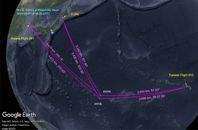
The main signal of interest at the early stage of the flight was recorded at H11S, with a bearing of \(269^{\circ }\), as shown in Fig. 12. Signals that appear to be generated by airguns are also observed, at a bearing of \(265^{\circ }\) relative to H11S. In addition, there are two earthquakes that erupted at time windows and locations related to the early stage of flight MH370. The first earthquake is a M 4.8–9 km South of Yōkaichiba, Japan, which erupted at 18:34:20 (UTC), on 7 March 2014. The earthquake epicentre is 3200 km away from H11S, which is a 36 min travelling distance for acoustic waves propagating at 1480 m/s. The bearing of the earthquake is \(311.83^{\circ }\) as calculated from the geographic locations, which well matches the calculated bearing from the signal, \({ 311.827^{\circ }}\) (see Fig. 16), with almost no deviation. The second earthquake is the M 2.7–85 km NE of Sinabang, Indonesia, erupted at 18:55:12 (UTC), on 7 March 2014. The earthquake epicentre is 3000 km away from H08S, which is a 34 min travelling distance for acoustic waves propagating at 1480 m/s. The bearing of the earthquake is \(67.12^{\circ }\) as calculated from the geographic locations. Due to the extremely high noise in the direction of \(210^{\circ }\), and since most of the energy in earthquake seem to be between 2.5 and 6 Hz filtering allows calculating a bearing of \(63.7^{\circ }\) with a relatively large deviation of \(3.3^{\circ }\) (see Fig. 17), which is about 140 km off the epicentre.
Figure 16 Bearing calculations of earthquake M 4.8–9 km S of Yōkaichiba, Japan, that erupted at 18:34:20 UTC on 7 March 2014 (Fig. 1). From top to bottom: recordings from three channels at station H11S between 19:05 and 19:15 UTC on March 7th 2014. Windowed entropy shows peaks (black triangles) where a transient signal is found. Each peak defines an event, for which bearing is calculated from differences in arrival times in the bearing subplot. The map demonstrates a perfect match with direction of the earthquake \(312^{\circ }\). Full size image