CaSSIS frost observations
We surveyed ~4,200 CaSSIS images (acquired up to 2022 February 05) with illumination geometries of 50–90° incidence within dusty, low thermal inertia (<100 TIU) regions (60° N—30° S). Only images that include the latest CaSSIS radiometric and absolute calibration were used in this study43,63,64.
The images used in this study consisted of early (6:00–9:00 lst) and late (15:00–18:00 lst) times. Analysis and comparison in these two local time regimes may help the distinction between early-morning and late-afternoon phenomena. During the survey, it was noticed that most CaSSIS images acquired at extremely high solar incidence angles of 85–90° contain colour and calibration artefacts due to the decrease in SNR and/or an increase in aerosol contribution from the atmosphere63. Consequently, the images with colour artefacts were labelled as ambiguous and were not used for further analysis.
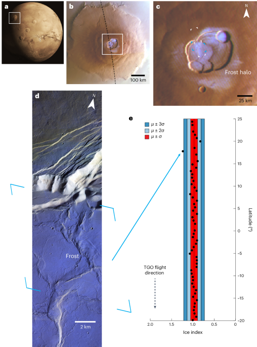
Frost detections relied on the use of CaSSIS NPB (near infrared (NIR) = 940, panchromatic (PAN) = 670, blue (BLU) = 497 nm) and synthetic RGB (red–green–blue; PAN and BLU only) products. These filter configurations allow a convenient separation between frosty and frost-free terrains. In CaSSIS colour products, frosty areas appear bluish, and/or whitish, and sometimes are bright only in the BLU filter (relative to frost-free areas; also see Supplementary Figs. 9 and 10). In support, we observe bluish frost deposits in HRSC colour images shown in Fig. 1b and Extended Data Fig. 1 (composites of blue (440 nm), green (530 nm) and red (750 nm) channels).
As shown by previous studies21,65 deposits are usually correlated with topography (prefer poleward-sloping terrains). Therefore, if both conditions were met (colour and topographic correlation), it was considered a strong indication of surface frost. As a final procedure, each of these candidate detections was then analysed using a spectral profile tool in the Environment for Visualizing Images software. This procedure extracts the pixel irradiance over flux (I/F) values between two manually selected points crossing the potentially frosted region in each filter. The profiles were then normalized by a mean I/F of a nearby frost-free, relatively flat region of interest (ROI), a well-established method to cancel out some of the atmospheric and topographic effects49,66,67,68,69,70. If the frost deposits were brighter in the BLU filter than the surrounding frost-free terrains by at least 3% (within CaSSIS absolute uncertainty43), then such images were flagged as potential frost detections. This survey yielded many frosty sites (not shown here) at latitudes ~40° N and ~30° S. However, because these latitude bands are dominated by known seasonal frost deposits21,23,65 and we do not have a robust method to distinguish between seasonal and diurnal frost, we further narrowed our filtering criteria. The final frost detections analysed here were restricted to equatorial ~20° N to ~10° S latitudes (outside of the seasonal mid-latitude regions). In this work, only equatorial sites that included visible evidence of frost are considered.
The spectral profile shown in Fig. 2e was computed by dividing each pixel along the profile by an average pixel value extracted from an ROI in Extended Data Fig. 5d. The ROI (>100 pixels in size) was selected on a frost-free and relatively flat terrain as suggested by the low slope values in the CaSSIS digital elevation model of this site. CaSSIS digital elevation models were produced by a pipeline developed at the Astronomical Observatory of Padova, National Institute for Astrophysics71,72.
NOMAD-LNO spectral processing
The NOMAD instrument is a suite of three high-resolution spectrometers also on board TGO, offering nadir infrared observations through its LNO channel37,73. This channel covers the 2.2–3.8 µm spectral range where several spectral features of ice are distributed over different wavelengths. Nevertheless, the NOMAD-LNO spectrometer has the particularity of not observing the entire spectral range at once. The data are acquired through small spectral windows, representing specific diffraction orders of the diffraction grating. Each LNO observation can select a maximum number of 6 diffraction orders every 15 seconds to ensure the best possible SNR74,75,76. The LNO footprint (instantaneous field of view) is 17.5 km × 0.5 km (ref. 75), which provides enough spatial scale to resolve the caldera of Olympus Mons. In this work, we use spectrally and radiometrically calibrated LNO data converted into a reflectance factor. The 2.7 µm ice band is the strongest in the LNO spectral range, resulting from both CO 2 and H 2 O ice absorption. Although the use of this band is not suitable for quantifying the amount of ice (easily saturated), it is effective for detecting homogeneous deposits (both CO 2 and H 2 O ice), as demonstrated with the ice index value77. This spectral parameter uses two diffraction orders. It is based on the combination of high reflectivity at continuum wavelengths with a more pronounced absorption in the 2.7 μm band. Initially defined as the spectral ratio between the reflectance factors of order 190 (continuum part, 2.32–2.34 µm) and 169 (short wavelengths shoulder of the 2.7 µm band, 2.61–2.63 µm) (ref. 77), we adjust the ice index by considering the available orders of the joint CaSSIS–NOMAD observations, that is, orders 190 and 168 (2.64–2.65 µm).
In nadir mode, the variability in the reflectance factors is caused mainly by the surface albedo variations resulting from the different absorption of the Martian surface mineralogy78,79,80. To remove spatial albedo variations over the explored Martian surface, we normalize the LNO reflectance factors to the Martian albedo. The adjusted ice index (II) can thus be defined as:
$${{\mathrm{II}}}=\frac{{R}_{2.33}}{{{{\mathrm{OMEGA}}}}_{2.32}}\div\frac{{R}_{2.63}}{{{{\mathrm{OMEGA}}}}_{2.62}}$$
where R i is the LNO reflectance factor value averaged around the central wavelength i of the LNO spectrum, fitted by a third-degree polynomial to mitigate the spectral oscillations resulting from the instrumental characteristics of the LNO channel, which become significant on the edges of each order (Supplementary Figs. 1 and 2). OMEGA i is the OMEGA albedo map80 based on reflectance spectra in the near infrared as NOMAD-LNO R i . Two OMEGA albedo maps are used in this work: one defined at 2.32 µm for order 190 and the other defined at 2.62 µm for order 168. Studies have shown that this spectral parameter identifies spatially extensive and abundant ice deposits when the index values are three sigma higher than their average value over ice-free mid-latitude terrain77,81.
Mars GCM modelling
We perform the Martian GCM simulation for the entire MY 36 using the MarsWRF model, which is the Mars adaptation of the general-purpose planetary atmosphere model, planetWRF47. Here the GCM set-up is based on a previous study46 examining the Martian planetary boundary and dust–turbulence interaction over a decade, from MY 24 to MY 34, which hosted three global dust storms. The reference model set-up46 was validated against NASA’s Mars Climate Sounder (MCS) observations on board the Mars Reconnaissance Orbiter, radio occultation observations from ESA’s Mars Express orbiter, as well as the in situ observations from NASA’s Mars Science Laboratory Curiosity rover. This model set-up consists of a semi-interactive two-moment dust transport model46 within the MarsWRF framework, in a way that the dust is lifted, mixed by model winds and sedimented, as guided by observed maps of column-integrated dust optical thickness82,83. Via this method, model processes govern the vertical dust distribution and related dust radiative heating, yet the horizontal dust distribution is guided to match the orbiter observations. In this model, the horizontal dust distribution is constrained to follow observations. In this model, the two-stream correlated k-distribution scheme is used for the short-wave and long-wave radiative transfer84. We use a Mars-specific boundary-layer turbulence parameterization scheme, which allows us to obtain the surface–atmosphere exchange coefficients85 Surface properties of the MarsWRF model, such as the topography, albedo, emissivity and thermal inertia, are acquired from the datasets of the Mars Orbiter Laser Altimeter2 and Thermal Emission Spectrometer (TES78) observations, where the details are presented in another study47. Here we increased the horizontal model grid spacing of the GCM from 5° × 5° to 2.5° × 2.5° (ref. 46), enabling better spatial coverage to provide more realistic boundary and initial conditions to our mesoscale simulations. We used 52 vertical sigma layers extending up to the model top of 100 km. The predicted surface temperatures are shown in Table 1.
Our modelling methodology is based on a previous study by MarsWRF85,86. Mesoscale simulations for Fig. 5 and Extended Data Fig. 7 were forced with initial and boundary conditions acquired by GCM simulations corresponding to the same seasonal conditions of CaSSIS observations shown in Figs. 1 and 2. The plots we present in terms of winds, pressure and temperature correspond to the local hours of observations. We nested three mesoscale domains in our GCM domain (see Supplementary Fig. 12 for details). Mesoscale domains use prescribed boundary conditions, derived either from GCM predictions (as in the case of d2) or from another mesoscale domain (d3 and d4). The GCM grid has a horizontal resolution of approximately 150 km. We progressively increased the horizontal resolution with a factor of three for our nested mesoscale domains. Our innermost domain, d4, has a horizontal resolution of 5.47 km. To assess the accuracy of our mesoscale predictions, we compared MarsWRF surface temperature predictions with the surface temperature observations by MCS and TES available for Olympus Mons and Arsia Mons regions at around 3:00 lst (Supplementary Fig. 13). We considered a sufficient Ls range of MCS and TES observations (Ls 310–360 for Olympus Mons and Ls 75–100 for Arsia Mons) to provide a sufficient set of observations to acquire a temperature map to be compared with MarsWRF simulations. These observations range from 1:00 lst to 4:00 lst, and MarsWRF estimations at the corresponding local times are compared for validation. The modelled surface temperatures for Olympus Mons caldera are within 10 K of the observations and within a few degrees Kelvin for Arsia Mons. It is important to note that these predictions carry uncertainties, particularly in regions with complex topography such as the Tharsis volcanoes.
Surface frost thickness and mass estimations
The MarsWRF GCM incorporates the phase transition and transport mechanisms of water vapour and ice, facilitating a parameterization of the Martian hydrological cycle that aligns with the methodologies outlined by previous studies87. This parameterization enables the model to approximate the surface frost layer thickness to about 1 μm at the locations in our study. However, it is important to acknowledge the inherent uncertainties associated with such estimations, particularly due to the limitations of physical parameterizations within Martian atmospheric models. These uncertainties are most pronounced in the prediction of atmospheric variables in regions lacking empirical observational data, such as the deposition rates of atmospheric volatiles.
In a recent experimental investigation, one study52 systematically evaluated the interaction between water frost deposition and the optical properties of a Martian soil simulant, specifically Mars Global Simulant (MGS-188). The experimental design involved the controlled deposition of water frost on the surface of the simulant, followed by precise measurements of both the spectral reflectance and the thickness of the frost layer. The findings indicate that a frost layer thickness ranging from approximately 10 to 20 μm is required to significantly attenuate the characteristic red slope of the spectral reflectance, aligning with the observed morning frost brightening in the blue wavelengths by approximately 10–20% as detected by the CaSSIS instrument. Furthermore, the study demonstrates that a relatively thin frost layer of about 100 μm is sufficient to flatten the visible spectrum, effectively neutralizing the spectral features.
Radiative transfer models50,51 can provide an additional constraint on the frost thickness estimation via the minimum optical depth (τ) necessary for frost visibility at CaSSIS visible and LNO near-infrared wavelengths. For example, with a τ of 10–2, we anticipate a minimal impact on albedo, less than 0.1 at CaSSIS visible wavelengths and negligible at LNO near-infrared wavelengths, given the single-scattering co-albedo is around 10−6 for visible light and less than 10−1 at 2.6 μm. However, LNO observations indicate a discernible albedo reduction at near-infrared wavelengths, suggesting a higher optical depth than 10−2. This implies that the frost’s grain radius and/or thickness must exceed 5 μm and 1 μm, respectively. If the grain radius is about 1 μm, then the frost layer’s thickness could be significantly greater, approximately 100 μm.
To conduct a preliminary quantification of the frost mass, we assumed a uniform frost layer thickness across all identified frost-covered regions, as observed by CaSSIS. The geographical extent of the frost coverage was approximated to the combined surface areas of the calderas of Martian volcanoes such as Arsia Mons, Olympus Mons, Ascraeus Mons and Ceraunius Tholus. By integrating the uniform frost thickness with the delineated area and adopting the density value for pure ice, we derived an initial estimate of the total frost mass. This approach provides a rudimentary yet insightful approximation of the frost mass, acknowledging the broad-scale estimative nature of this calculation.
Boulder size measurements
To investigate a potential effect of the diurnal frost cycle on the overall geomorphology and landscape evolution, we studied the shape of mass-wasted boulders across six sites of interest. Here we compare the sizes of boulders on volcanoes with frost as determined by CaSSIS (two sites in Olympus Mons and one in Arsia Mons) and on volcanoes where frost has not been detected (Tharsis Mons, Jovis Tholus and Ulysses Tholus). Because frost accumulates preferentially on poleward-facing slopes on Mars29, here we focused only on north-facing and south-facing slopes. This might reveal whether there are considerable differences in boulder sizes due to frost weathering89.
We used eight map-projected High Resolution Imaging Science Experiment (HiRISE)90 images in Geographic Information System (QGIS) to determine the three principal dimensions of each identified boulder. The first dimension is defined as the longest distance between two points on the boulder as visible from orbit. Similarly, the second dimension is defined as the diameter of the boulder orthogonal to the first dimension. Last, the third dimension is defined as the height of the boulder as estimated using shadow length and solar incidence angle. In total, we identified and measured 63 boulders across the six sites. All derived measurements were plotted on ternary diagrams91 using the Tri-Plot software92. These diagrams relate the three principal dimensions of each boulder, visualizing its overall shape as well as similarities and differences within and across the studied sites.