Local Lynx of Cold Clouds
We show below that the distance and velocity characteristics of the LRCC are such that there is at least a 1.3% chance that the heliosphere encountered the tail of the LRCC 2 million years ago (Ma) in the direction of the Lynx constellation. We name that portion the Local Lynx of Cold Clouds (LxCCs). The LxCCs represent nearly half of all the mass of the LRCC and are more massive than the more well-studied LLCC, presuming an identical distance. The LRCC has a very placid and smooth velocity field, and it is a thin band that stretches across nearly 90° of the sky. Taking advantage of this remarkably well-organized velocity structure, Haud6 modelled it as a subarc of a rotating, expanding, moving ring in space with five parameters. Here we propose a more modest, three-parameter model, in which the LRCC simply moves as a fixed, non-rotating structure, and solve for the full three-space motion of the cloud. We use 21 cm data from the all-sky HI4PI survey (HI4PI Collaboration10), from which we isolate cold structures and fit with narrow-line Gaussians. We recover spatial and velocity structures consistent with the results Haud6 recovered from a lower-resolution dataset. We fit the velocity field as a fixed, non-rotating structure. The relative velocity in Galactic coordinates between the LLCC and the Sun is (∆U, ∆V, ∆W) = (−13.58, −1.40, 3.70) km s−1 or a velocity of 14.1 km s−1 towards l = 186° and b = 15° (l is Galactic longitude and b is Galactic latitude). We found that the 1σ error region of the direction of flow of these clouds covers 1.3% of the sky (576 square degrees), including the tail of the LRCC itself (Figs. 1 and 2). This probability could be larger because the LRCC is a wide structure that spans a large portion of the sky. As shown in Fig. 3, in our Monte Carlo simulation, the LRCC as a whole is wildly unstable in the ISM, and thus, it was probably larger in the past. So, the low chance of collision is a lower limit.
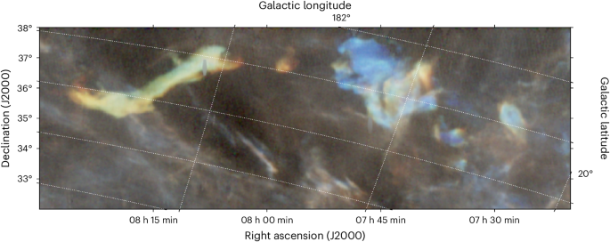
Fig. 1: Zoom-in of the LxCCs as seen in 21 cm data from the GALFA-HI survey. In this visualization, three 21 cm velocity channels, each 0.786 km s−1 wide, are mapped to red, blue and green. Red represents 8 km s−1, green 8.7 km s−1 and blue 9.5 km s−1, all in the local standard of rest (LSR) frame. The scale is logarithmic from 2 to 40 K brightness temperature. The visualization technique is designed to make the cold clouds stand out in colour (green and red for the left component and iridescent blue for the right component) by taking advantage of the narrowness of their velocity profiles compared to the warmer background gas much farther away. GALFA-HI survey data from ref. 67. Full size image
Fig. 2: Cartoon of the LRCC and its three-dimensional velocity. We show the LRCC with two LxCCs highlighted in red. The Sun is shown in the Galactic plane at (0,0), with a 10 pc grid for scale. The black dashed line represents the path of the Sun in the LRCC rest frame. The grey dashed lines represent the 68% confidence interval of the past path of the Sun, which contains only 1.3% of the total sky. Full size image
Fig. 3: The collision between the LxCCs and the Sun is shown in the LSR frame using an interactive graphic. For this plot, 100 draws made from the velocity and distance distributions were tracked backwards in time. Each red point represents the path of the LxCCs from 5.75 Ma to the present. The dotted yellow line is the velocity field of the Sun. The blue surface represents the edge of the Local Bubble64 (Supplementary Video 1). Credit: Catherine Zucker (https://faun.rc.fas.harvard.edu/czucker/Paper_Figures/Interactive_LxCC.html). Full size image
As the clouds have a positive (outgoing) velocity, the coincidence of the cloud on the sky within the cloud velocity error circle indicates that the Sun crossing the clouds is consistent with the model. The distance to the LLCC, the largest cloud in the LRCC, is known to be between 11 and 45 pc, which allows us to compute a 68.3% confidence interval for the LxCCs of 22 to 59 pc (‘LLRC detection, distance and velocity statistics’ in Methods). We found the 68.3% confidence interval of the radial velocity to be 11.4–15.6 km s−1. These parameters translate to the Sun crossing the position of the clouds between 1.57 and 4.2 Ma. It, therefore, appears compelling that the Solar System passed through a cold, dense, ISM cloud 2 Ma (Fig. 3). Note that these clouds are anomalous and unexplained structures in the ISM, and their origin and physics are not well understood8. We have assumed here that these clouds have not undergone any substantial change over the last 2 Myr, though future work may provide more insight into their evolution.
Heliosphere 2 Ma
We simulated the interaction of the heliosphere 2 Ma with the LxCCs. The distance to the edge of the heliosphere is currently ~130 au, as measured by Voyagers 1 and 2 (ref. 11). As our simulation demonstrates, the momentum deposition by the large hydrogen density of the cloud shrinks the heliosphere to a scale that is much smaller than the Earth’s orbit around the Sun and brings the Earth and the Moon in direct contact with the cold ISM. Such an event may have had a dramatic impact on the Earth’s climate.
Our computational code considers a single ionized component and four neutral components12, although for this run, we used only the ISM component, which is orders of magnitude more abundant than the heliosheath and supersonic solar-wind components. We used inner boundary conditions for solar-wind conditions at 0.1 au (or 21.5 solar radii). The parameters adopted for the solar wind were based on the well-benchmarked Alfven-driven solar-wind solution13. The grid was highly resolved at 1.07 × 10⁻³ au near 0.1 au and 4.6 × 10⁻³ au in the region of interest, including the tail (Supplementary Fig. 1). The run was performed for 44 years (see ‘Description of the numerical model’ in Methods for a description of the coordinate system, grid and model details). For the ISM outside the heliosphere, we adopted the characteristics of the LLCC8, namely, n H = 3,000 cm−3 and T = 20 K. We included a negligible ionized component (n i = 0.01 cm−3 and T = 1 K) and ignored the interstellar magnetic field as its pressure is negligible compared to the ram pressure of the cold cloud. We adopted the relative speed between the Sun and LxCCs \((\Delta U,\Delta V,\Delta W\;)=\left(-13.58,-\mathrm{1.40,3.70}\right)\) km s−1 or a velocity of 14.1 km s−1. We rotated the system so that the flow is in the z–x plane with the ISM approaching from the -x direction. The neutral H from the cold cloud impinged on the heliosphere with speeds of U x = 14.1 km s−1, U y = 0 km s−1 and U z = 1.1 km s−1 (see ‘ISM conditions’ in Methods for details).
The numerical model includes charge exchange between the neutrals and ions12, as well as the Sun’s gravity, which plays an important role in focusing the gas flow. Neutral H atoms are included through a multi-fluid description that is appropriate for the high densities14,15. Two fluids are used, one between the pristine ISM and the bow shock that forms ahead of the heliosphere and one that captures the heated and decelerated population between the bow shock and the heliopause (HP). We neglected radiation pressure from the Lyα line of hydrogen atoms since these cold dense clouds are optically thick to Lyα photons4. We neglected photoionization, as its contribution is an order of magnitude smaller than that of charge exchange at these distances (see ‘Description of the numerical model’ in Methods for details).
Figures 4 and 5 show the heliosphere as a result of the interaction with LxCCs 2 Ma. The heliosphere shrinks to 0.22 ± 0.01 au, which is well within the Earth’s orbit, thus exposing the Earth (and all the other Solar System planets for most of their trajectories) to the ISM, which has neutral densities of 3,000 cm−3 (Fig. 6c). Due to gravity, the neutral density increases as the cold cloud encounters the heliosphere, so that inner planets, such as Mercury and Venus (at distances of 0.39 and 0.72 au), will encounter densities of 7,000 cm−3. The size of the heliosphere can be compared with the stand-off distance expected from analytic estimations. One can estimate analytically the stand-off distance16 as approximately \({r}_\mathrm{E}\sqrt{{\rho}_\mathrm{E}{v}_\mathrm{E}^{2}/{\rho}_{\infty }{v}_{\infty }^{2}}\), where r E , v E and ρ E are the radius, speed and density of the solar wind at Earth and ρ ∞ and v ∞ are the density and speed at infinity of the ISM. Taking the values ρ E = 5.71 cm−3, v E = 417 km s−1, ρ ∞ = 3,000 cm−3 and v ∞ = 14.1 km s−1, the stand-off distance is 1.3 au. The neutral density due to gravity increases to 10,000 cm−3 ahead of the heliosphere and the neutral speed to 50 km s−1, making the same estimate 0.2 au, which agrees very well with the simulation results.
Fig. 4: Three-dimensional image of the heliosphere. a,b, Side view in (x,z) coordinates (a) and top view in (x,y) coordinates (b) (‘Description of the numerical model’ in Methods). The orbit of Earth around the Sun is plotted in red. The isosurface of the heliosphere is plotted with speed of 100 km s−1. We plotted the tail out to 4 au. Full size image
Fig. 5: View of the heliosphere 2 Ma. The heliosphere at the end of the simulation at 44 years in the meridional plane at y = 0 au (for the model coordinate system, see ‘Description of the numerical model’ in Methods). Contours are speed. The heliosphere shrinks to 0.22 au at the nose. It maintains a long cometary shape and exposes all the planets to the cold dense ISM material. Full size image
Fig. 6: A closer view of the heliosphere 2 Ma. This figure provides a closer view of Fig. 5. Panels are shown at the end of simulation at 44 years in the meridional plane at y = 0. The coordinate system is such that the z axis is parallel to the solar rotation axis, the x axis is oriented in the direction of the interstellar flow (which points 5° upward in the x–z plane) and the y axis completes the right-handed coordinate system where the Sun is at rest at the centre. a, Magnetic field. b, Ion density. c, Neutral density. d, Speed. Full size image
The supersonic solar wind goes through a termination shock (TS; Fig. 5) before reaching equilibrium with the cold cloud. The heliosphere has a cometary shape with a long tail (Fig. 5) that is unstable. Due to their short mean free path (~0.01–0.1 au), the neutrals are quickly depleted across the HP (Fig. 6c), setting a strong gradient for the ram pressure. The heliosphere reaches equilibrium with the cold cloud at the HP between the compressed solar magnetic field and the ram pressure of neutrals ahead of the HP (Supplementary Fig. 2). Gravity increases the density from 3,000 cm−3 and the speed from 14.1 km s−1 of neutrals at large distances to 10,000 cm−3 and to 50 km s−1, respectively, near the HP (Fig. 6c,d).
A bow shock is formed in the ISM (Fig. 6d). The density of neutrals increases to ~10,000 cm−3 near the bow shock. In that region, the temperature also increases to ~105 K. The cooling time τ cooling for different densities and temperatures17 varies in the range log 10 [τ cooling (s)] ≈ 10–15. The lower limit on the cooling time is ~300 years, which is much longer than the dynamic time to form the shock τ dyn . For the relative speed with which the Earth moves through the ISM, namely, 27 km s−1 ≈ 6 au yr−1, and a bow shock thickness of about less than 1 au, it follows that τ dyn ≈ 1 year, which is much shorter than τ cooling . Hence, radiative losses can be neglected.
The heliosphere 2 Ma was very different from the heliosphere of today12. There was no hydrogen wall as the number of ions ahead of the heliosphere was negligible. The heliosphere was so close to the Sun that the solar magnetic field was radial (Fig. 6a) and the heliosheath plasma confinement (Fig. 6b) did not take place12. The flow in the heliosheath was fast (~110–260 km s−1) (Fig. 5), and the ram pressure was larger than the magnetic pressure. The Rayleigh–Taylor-like instability that currently occurs in the heliosheath18 and drives the current heliosphere to have a short tail was absent. Because of the short mean free path, there were almost no neutrals inside the heliosheath, and the density gradient in the heliosheath was absent as well. The TS shifted to distances as close as 0.12 au from the Sun. The present-day TS is weakened by pickup ions compared to the much stronger compression ratio of 3.7 of the TS during the passage of the cold cloud. This has consequences for accelerating particles to high energies. We expect that the stronger shock accelerated particles more efficiently than the current TS, which is mediated by pickup ions19. Future work is needed to explore the resulting non-thermal emission and its consequences for planets around the Sun and other stars.
Figure 5 shows the elongated, high-speed tail of the ancient heliosphere. Such elongated tails may be common for solar-mass stars just born in dense interstellar environments, like molecular clouds, and they may have been misinterpreted in the past as jets20.
60Fe and 244Pu isotopes
By studying geological radioisotopes on Earth, we can learn about the past of the heliosphere. 60Fe is predominantly produced in supernova explosions21 and becomes trapped in interstellar dust grains. 60Fe has a half-life of 2.6 Myr, and 244Pu has a half-life of 80.7 Myr. 60Fe is not naturally produced on Earth, and so its presence is an indicator of supernova explosions within the last few (~10) million years. 244Pu is produced through the r-process that is thought to occur in neutron star mergers22. Evidence for the deposition of extraterrestrial 60Fe onto Earth has been found in deep-sea sediments and ferromanganese crusts between 1.7 and 3.2 Ma (refs. 23,24,25,26,27), in Antarctic snow28 and in lunar samples29. The abundances were derived from new high-precision accelerator mass spectrometry measurements. The 244Pu/60Fe influx ratios are similar at ~2 Ma, and there is evidence of a second peak at ~7 Ma (refs. 23,24). In addition, cosmic ray data assembled by the Advanced Composition Explorer spacecraft measured the 60Fe abundance as well30. This study estimated the time required for transport to Earth and concluded that the cosmic rays diffused from a source closer than a distance of thousands of parsecs. Studies have attributed the two peaks in 60Fe to supernova explosions within 100 pc over the last 10 Myr that formed the Local Bubble24. Processes that brought 244Pu to Earth include supernova ejecta.
Other studies suggest that nearby supernova explosions within ~10–20 pc could have produced the above isotopes31. In particular, the heliosphere would collapse to distances less than 1 au if a supernova is closer than 10 pc. This scenario requires fine-tuning, as this distance is very close to the so-called kill radius of 8 pc (ref. 32), the distance necessary to initiate a mass extinction. A close supernova explosion contradicts the recent model of the Local Bubble formation33, which indicates that the Local Bubble originated when supernovae exploded 14 Ma near the centre of the Local Bubble at a distance much larger than 10 pc. For supernovae at further distances (such as the more recent study34 that places a supernova at 50 pc), it has yet to be shown that sufficient 60Fe can be deposited onto Earth if 60Fe is embedded in large interstellar dust grains, although some researchers35 have started to investigate this (albeit the complex filtration of the heliosphere and its magnetic field affecting its propagation to Earth has yet to be investigated). In particular, the propagation of dust in a realistic heliospheric magnetic field has yet to be studied. Our proposed scenario agrees with the geological evidence from 60Fe and 244Pu isotopes that Earth was in direct contact with the ISM during that period.