Introduction
The goal of this post is to determine how the latency is going to be impacted if the service time is going to be cut in half. I was watching a great presentation of Martin Thompson where he mentioned this example example and wanted to freshen up my queuing theory a bit and do some calculations.
Lots of formulas
Let’s first get some formulas out of the way.
The mean latency as function of the utilization:
\(R\) is latency (residency time)
\(\mu\) is service rate
\(\rho\) is utilization
\[R=\dfrac{1}{\mu(1-\rho)}\]
\(\mu\) is the reciprocal of service time \(S\).
\[\mu=\dfrac{1}{S}\]
And if we fill this in and simplify the formula a bit, we get the following:
\[R=\dfrac{1}{\dfrac{1}{S}(1-\rho)}\] \[R=\dfrac{S}{(1-\rho)}\]
Another part we need is the calculation of the utilization:
\(\rho\) is the utilization
\(\lambda\) is the arrival rate.
\(S\) is the service time.
\[\rho = S \lambda\]
This formula is known as the Utilization Law or Little’s Microscopic Law.
And this can be converted into a function that calculates the arrival rate as a function of utilization and service time:
Comparing the latencies
\[\lambda = \dfrac{S}{\rho}\]
In Martin’s example he has 2 services:
an unoptimized service with \(S=0.1\) seconds.
an optimized service with \(S=0.05\) seconds
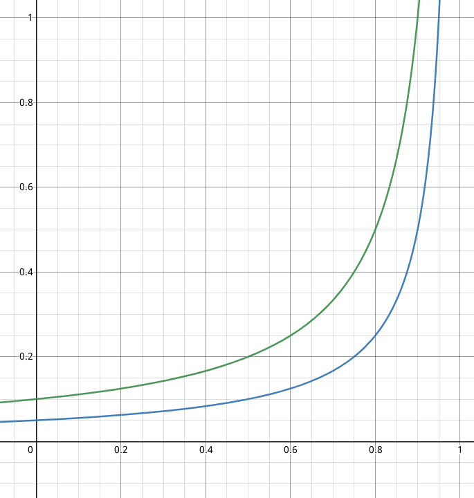
To make it a bit more tangible let’s plot latency curves as function of utilization for both services.
green: unoptimized service
blue: optimized service
The x-axis is the utilization and the y-axis is the latency.
The first thing we can calculate is the latency with a service time of 0.10 seconds and a utilization of 0.90 because this utilization Martin picked in his example:
\(R=\dfrac{S}{(1-\rho)}=\dfrac{0.10}{(1.0-0.90)}=1.0\) second.
The next part we need to determine is the arrival rate based on the utilization and service time. So with a service time of 0.10 and a utilization of 0.90 we get the following arrival rate:
\(\lambda = \dfrac{S}{\rho} = \dfrac{0.1}{1-0.9} = 10\) requests/second.
So if the service time is going to be cut in half, and we keep the same arrival rate, the utilization is going to be cut in half:
\[\rho = S \lambda = 0.05 \times 10 = 0.45\]
And if fill this into the calculate the latency is function of the utilization for the optimized service, we get:
\(R=\dfrac{S}{(1-\rho)} = \dfrac{0.05}{1-0.45}=0.091\) seconds.
We can see both the calculated latencies in the plot below:
So we went from a latency of 1 second to 0.091 seconds which is an \(\dfrac{1}{0.091}=11\) times improvement.
Discrepancy
Martin’s claim is that the latency improvement is 20x. But the results based on the above formulas don’t agree with that. He makes a remark that the unit of processing is half the calculated latency, but I don’t understand what he means or how this is relevant for the latency calculation.
I haven’t configured comments yet on this new website. So if you want to comment, send me a message on Twitter.