Samples
Data were obtained from four studies: International Study to Predict Optimized Treatment in Depression (iSPOT-D18, https://clinicaltrials.gov/ct2/show/NCT00693849), Research on Anxiety and Depression study (RAD38), Human Connectome Project for Disordered Emotional States (HCP-DES39) and Engaging self-regulation targets to understand the mechanisms of behavior change and improve mood and weight outcome (ENGAGE40, https://clinicaltrials.gov/ct2/show/NCT02246413). Clinical participants from these studies (n = 801) represented the full spectrum of severity of depression and anxiety disorders (see Table 1 and Supplementary Table 1 for details). Healthy controls (iSPOT-D, n = 67; HCP-DES, n = 70) were used as a reference group for building regional circuit scores from the imaging data (see below). Of the 801 clinical participants, 250 completed randomized controlled trials of either antidepressant pharmacotherapy for major depressive disorder (n = 164)18 or behavioral intervention for clinically substantial depressive symptoms and obesity (n = 86)40 (see Supplementary Table 2 for more details).
All participants provided written informed consent. Procedures were approved by the Stanford University Institutional Review Board (IRB, protocol nos. 27937 and 41837) or the Western Sydney Area Health Service Human Research Ethics Committee.
MRI acquisition and preprocessing
Details of MRI sequences, fMRI tasks, MRI data quantification and quality control are given in Supplementary Methods.
Acquisition
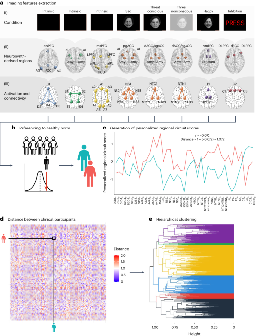
Participants underwent the Stanford Et Cere Image Processing System protocol, which probes six brain circuits: default mode circuit, salience circuit, attention circuit, negative affect circuit, positive affect circuit and cognitive control circuit17,20. The Facial Expressions of Emotion Tasks probed the positive and negative affect circuits and a Go–NoGo task probed the cognitive control circuit. We derived measures of task-free function of the default mode, attention and salience circuits from the task data41,42. Task-free measures were independent of those obtained from the task conditions (Supplementary Fig. 14).
Preprocessing
The MRI data were preprocessed using fMRIprep43. We discarded scans if they contained incidental findings, major artifacts or signal dropouts or had >25% of volumes containing significant frame-wise displacement. An experienced rater (L.T.) also visually checked each scan, leading to the exclusion of 32 participants. Scans removed owing to excessive motion were: Go–NoGo task = 38, Conscious Facial Expressions of Emotion Task = 92, Non-conscious Facial Expressions of Emotion Task = 76 and task free = 51 (see Supplementary Table 17 for the number of scans passing criteria).
Derivation of regional circuit scores
A summary of how regional circuit scores were obtained is given in the following sections (Fig. 1; see Supplementary Methods for details). We previously demonstrated that this system produces valid and clinically useful individual circuit clinical scores20.
Extraction of imaging features of interest
The regions of interest within six circuits of interest were defined from the meta-analytic platform Neurosynth44 (see Supplementary Table 18 for search terms and coordinates) and refined by removing regions that did not pass quality control or psychometric criteria. Of the remaining regions, we only retained 29 regions implicated in our theoretical synthesis of dysfunctions in depression and anxiety20,38. From these regions, we derived 41 features of activation, task-based and task-free connectivity for subsequent analyses20 (see Supplementary Table 18 and Supplementary Tables S5A and S5B in ref. 20 for details on the regions of interest and features). Our focus on regions defined from theory, meta-analyses and anatomy can lead to reliable and reproducible imaging measures. For example, activations within anatomically defined regions of interest have acceptable-to-high within-participant reliability45, as does connectivity within established brain networks46.
All following analyses used RStudio 2022.07.2, R v.4.1.3. Code for these analyses and the regions of interest to derive our imaging features are at https://github.com/leotozzi88/cluster_study_2023.
Imputation of missing values
As a result of missing scans and quality control, some regional circuit scores could not be computed for some participants: 7.57% for the default, salience and attention scores, 9.38% for the negative affect sad scores, 9.38% for the negative affect threat conscious scores, 6.72% for the negative affect threat nonconscious scores, 4.05% for the cognitive control scores and 9.38% for the positive affect scores. We imputed these values separately for each scanner by using multiple imputation by chained equations with random forests (R package miceRanger), using one iteration of a predictive mean matching model with the imaging features as the input.
Correction for scanner effects
We removed the potential confounding effect of between-scanner variability using ComBat47,48,49, an established method that uses an empirical Bayesian framework to remove batch effects.
Referencing to a healthy norm
All imaging features of the clinical participants were expressed in s.d. units relative to the mean and s.d. of healthy controls. These values are henceforth referred to as ‘regional circuit scores’ and represent the amount of dysfunction of each component of each circuit. Subsequent analyses were conducted on the regional circuit scores of the clinical participants only.
Symptom measures
We used self-reported questionnaires to operationalize: ruminative worry (Penn State Worry Questionnaire—Abbreviated total50); ruminative brooding (Ruminative Response Scale total51); anxious arousal (Mood and Anxiety Questionnaire general distress subscale52); negative bias (Depression Anxiety and Stress Scale (DASS) depression subscale); threat dysregulation (DASS anxiety subscale); anhedonia (Snaith–Hamilton Pleasure Scale total53); cognitive dyscontrol (Barratt Impulsiveness Scale attentional impulsiveness subscale54); tension (DASS stress subscale); insomnia (Quick Inventory of Depressive Symptomatology—Self-Report Revised (QIDS-SR) sum of items 1–3 (ref. 55)); and suicidality (QIDS-SR item 12). In iSPOT-D, we used the Hamilton Depression Rating Scale (HDRS) total score as a measure of depression severity56 and, in ENGAGE, we used the Symptom Checklist 20 Depression Scale (SCL-20)57. See Supplementary Table 19 for the participants in each sample available for each measure.
Clinical diagnoses
DSM-IV-TR (RAD), DSM-5 (HCP-DES) or DSM-IV (iSPOT-D) criteria for major depressive disorder, anxiety disorder, post-traumatic stress disorder or obsessive–compulsive disorder were ascertained by a psychiatrist, general practitioner or researcher using the structured MINI34. In ENGAGE, patients were considered eligible if they scored ≥10 on the PHQ-9, a threshold with 88% specificity for major depressive disorder35, and had a qualifying body mass index (BMI). Comorbidities were ascertained from electronic health records.
Behavioral performance measures
Cognitive performance was assessed using WebNeuro37,58,59. We focused on the tests for which our regional circuit scores have been shown to predict performance20: sustained attention (omission errors, commission errors and reaction times in a continuous performance test); executive function (errors and completion time of a maze test); cognitive control (commission errors and reaction times in a Go–NoGo test); explicit emotion identification (reaction time to identify happy, sad, fearful and angry faces); and implicit priming bias by emotion (difference in reaction time in a face identification task when primed implicitly by happy, sad, fearful and angry faces compared with neutral faces). For analyses, we used the test performance referenced to an age-matched norm generated by WebNeuro (z-scores). See Supplementary Table 19 for the number of participants in each sample available for each measure.
Treatment
In iSPOT-D, participants were randomized to one of three treatments: escitalopram (selective serotonin reuptake inhibitor (SSRI)), sertraline (SSRI) or venlafaxine XR (selective serotonin–norepinephrine reuptake inhibitor (SNRI))18. In ENGAGE, participants were randomized to either a behavioral intervention combining problem-solving, behavioral activation and weight loss (Integrated Coaching for Better Mood and Weight, I-CARE) or usual care (U-CARE)19,40. No treatment was administered in HCP-DES and RAD, so these studies were not considered in the treatment analyses.
Identification of depression biotypes
To identify biotypes within our clinical participants, we used hierarchical clustering of their 41 regional circuit scores. We selected the optimal number of clusters using six convergent sources of evidence: the elbow method; two procedures proposed by Dinga et al.14 to evaluate biotypes of depression (simulation-based significance testing of the silhouette index and stability using crossvalidation); permutation-based significance testing of the silhouette index; split-half reliability of the cluster profiles; and the match of the solution to a theoretical framework17 (Fig. 2).
Hierarchical clustering
For each pair of clinical participants, we first computed the correlation coefficient of their 41 imaging-derived regional circuit scores (Fig. 1). Then, we computed the dissimilarity between each pair of clinical participants as 1 − this correlation (see ref. 60 for a similar approach). We used the between-individual dissimilarity matrix as input to hierarchical clustering using the average as agglomeration method.
Elbow method
The first source of evidence that we used to choose the optimal number of clusters was the elbow method, based on a plot showing the within-cluster sum of distances between participants for solutions between 2 and 15 clusters (Fig. 2a).
Simulation-based significance testing of silhouette
We tested the probability of our observed average silhouette index occurring under the null hypothesis of no clusters (that is, of the data coming from a multinormal distribution)14. For clusters between 2 and 15, we conducted 10,000 simulation runs, in which we drew 801 participants from a multinormal distribution that had the same mean and covariance for each regional circuit score as our data. These simulated participants were then used as input in hierarchical clustering, as described above, and the average silhouette index across participants was calculated. Thus, we obtained null distributions for these average silhouette indices. Finally, we calculated the proportion of average silhouette indices generated under the null that were greater than the one we obtained from our data (P value). We considered statistically significant solutions with numbers of clusters for which P < 0.05 (Fig. 2b).
Permutation-based significance testing of silhouette
For each number of clusters between 2 and 15, we shuffled each brain circuit score across subjects 10,000×, then repeated the hierarchical clustering as described above and calculated the average silhouette index. Thus, we obtained null distributions for these average silhouette indices. Finally, we calculated the proportion of average silhouette indices generated under the null that were greater than the one we obtained from our data (P value). We considered statistically significant solutions with numbers of clusters for which P < 0.05 (Fig. 2c).
Assessment of cluster stability using crossvalidation
To evaluate whether the clustering was stable under small perturbations to the data14, we repeated the clustering procedure 801×, each time with one participant left out. For each run and for each solution between 2 and 15 clusters, we calculated the similarity of the new cluster assignments to the original ones using the ARI (Fig. 2d). We then repeated this procedure while holding out 20% of the sample instead of one participant (Fig. 2e).
Matching of clusters to a theoretical framework
We identified the primary circuit dysfunction of each cluster by averaging the values of regional circuit scores by circuit and modality (task-based activity, task-based connectivity, task-free connectivity) and identifying the measures that showed a >0.5 s.d. absolute mean difference compared with the healthy norm. We then compared the profile of circuit dysfunction of each cluster with those hypothesized in a theoretical framework of circuit dysfunction in depression and anxiety16,17.
Split-half replication of cluster profiles
First, we split our dataset into two random samples of equal size. Then, we ran our clustering procedure on the first half-split. Then, we assigned each participant in the second split to one of the clusters obtained in the first half-split. To do so, we computed the mean circuit scores across all participants belonging to each cluster in the first half-split. Then, we calculated Pearson’s correlation coefficient between each participant’s brain circuit scores and these cluster-averaged scores. Each out-of-sample participant was assigned to the cluster for which this correlation was highest. Finally, we identified the primary circuit dysfunctions of each cluster in each split as described above (>0.5 s.d. absolute mean difference compared with the healthy reference data) and examined whether they replicated the circuit profiles found in the whole sample visually and by computing Pearson’s correlation coefficient of the mean profile dysfunction profile of each cluster between splits (Fig. 2f).
Clinical characterization of biotypes
We characterized our final clustering solution by using external clinical measures independent of cluster inputs: symptoms, clinical diagnoses, performance on behavioral tests and treatment response. Importantly, we also replicated our findings in split-half and leave-study-out analyses (Fig. 2g–l).
Comparison of symptoms between biotypes
For each symptom, we compared the median severity of participants in each biotype to the median severity of participants who were not in the biotype using Wilcoxon’s tests. As insomnia and suicidality were assessed using only three and one QIDS-SR items, respectively, we used a χ2 test to compare the fraction of participants in the biotype who endorsed any of the items (total value >0) compared with participants who were not in the biotype. For Wilcoxon’s tests, we calculated the effect size r as the z statistic divided by the square root of the sample size and we considered significant tests for which P < 0.05 (Fig. 2h,j).
Comparison of behavioral performance between biotypes
For each of our behavioral performance measures, we compared the median performance of participants in each biotype with the median performance of participants who were not in the biotype using Wilcoxon’s tests. We calculated the effect size r as the z statistic divided by the square root of the sample size and we considered significant tests for which P < 0.05 (Fig. 2i,k).
Comparison of treatment response between biotypes
To obtain a comparable measure of symptom severity across our clinical trial datasets, we first scaled the measures of total HDRS scores (collected in iSPOT-D) and SCL-20 scores (collected in ENGAGE) between 0 and 1 based on the minimum and maximum values of each scale. We defined response as a decrease of at least 50% of symptom severity from baseline to follow-up and remission as follow-up HDRS ≤ 7 or SCL-20 ≤ 0.5. Then, for each treatment modality and each biotype, the severity of symptoms after treatment of participants in the biotype was compared with the median symptom severity of clinical participants not in the biotype using Wilcoxon’s tests. For these tests, we excluded biotypes in which only five or fewer participants received a treatment. We calculated the effect size r as the z statistic divided by the square root of the sample size and considered significant tests for which P < 0.05. (Fig. 2l).
Split-half replication of clinical associations
We replicated the significant comparisons of behavior and symptoms between biotypes found in the complete sample by splitting the sample into two random halves, repeating the clustering procedure on the first half and then assigning participants in the second half to the clusters obtained in the first half, as described above. We then conducted Wilcoxon’s tests as described above in each split and considered a result replicable if it was significant both in the original sample and in each of the split-half samples (for the second split, we conducted a confirmatory one-sided test).
Leave-study-out replication of clinical associations
For each of the four studies included in our dataset, we replicated the significant comparisons of behavior and symptoms between biotypes by splitting the sample into two subsets: one containing the participants who were not from that study and one containing participants from that study. Then, we repeated the clustering procedure on the first split and assigned participants in the second subset to the clusters obtained in the first split, as described above. We then conducted Wilcoxon’s tests as described above and considered a result replicable if it was significant in each of the two splits when holding out at least one study (for the second split, we conducted a confirmatory one-sided test).
Comparison of diagnoses between biotypes
To evaluate whether the clusters reflected traditional diagnostic categories, we used χ2 tests to compare the proportion of clinical participants in each biotype who met criteria for major depressive disorder, generalized anxiety disorder, obsessive–compulsive disorder, post-traumatic stress disorder, panic disorder or social phobia.
Comparison of covariates of no interest between biotypes
To verify that biotypes were not driven by scanner effects, we used χ2 tests to evaluate whether the proportion of participants in each cluster was different across scanners. Similarly, we used χ2 tests to examine the effects of gender and dataset and a one-way analysis of variance (ANOVA) to test whether different biotypes had different age distributions.
Comparison of brain circuit scores to other biotyping inputs
We selected three alternative feature sets, each used in a recent paper identifying biotypes of depression using resting state fMRI (to our knowledge, no prior publication has used task fMRI): whole-brain functional connectivity from the Power atlas4; functional connectivity in the default mode network5; and a functional connectivity of the angular gyrus7. We evaluated these features using the same criteria that we used for our own: (1) solution outperforms null hypothesis of no clusters (simulated data); (2) solution outperforms null hypothesis of no clusters (permuted data); (3) ARI (leave-one-out mean); (4) ARI (leave-20%-out mean); (5) generalizable cluster profiles across random split-half; (6) generalizable symptom differences across random split-half; (7) generalizable behavior differences across random split-half; (8) generalizable symptom differences across leave-study-out; (9) generalizable behavior differences across leave-study-out; and (10) biotypes differ in treatment response. For each of the alternative sets of features, we evaluated the number of clusters reported in the original paper and six clusters (the number that we chose in our analysis). We also conducted two statistical tests comparing clustering performance using our features with other features. First, a resampling test: we sampled 80% of participants, used each set of features to cluster their data and computed the corresponding average silhouette index over 10,000 iterations. For each set of alternative features, we considered as P resample the fraction of samplings in which the silhouette index was higher than the one obtained with our features. Then a permutation test: after clustering each of the imaging feature sets, we randomly permuted the cluster assignments 10,000× and computed a silhouette score for each. This provided us with null distributions of the silhouette index for each feature set. We then calculated the difference between the null distribution of the silhouette index obtained using our features and each of the null distributions obtained from alternative features. We considered as P permute the proportion of permutations in which the difference between the two null distributions was greater than that between the silhouette indices of the real solutions. We considered our features to provide a better clustering when P permute < 0.05 and P resample < 0.05.
Finally, we compared our original results to results obtained using only our task-free brain circuit scores, choosing as the number of clusters six (the number we chose in our analysis using all features) and two (the number of clusters with task-free dysfunction identified in our analyses).
Reporting summary
Further information on research design is available in the Nature Portfolio Reporting Summary linked to this article.