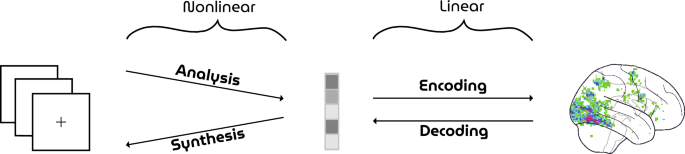
HYPER pipeline
An illustration of the HYPER pipeline can be found in Fig. 2. Visual face stimuli were synthesized by the generator network of a GAN and presented to participants in an fMRI scanner. Neural decoding was performed as follows: the generator network of the GAN was extended with a dense layer at the beginning of the network that performed the response-feature transformation (i.e., from voxel recordings to latent vectors). This response-feature layer was trained by iteratively minimizing the Euclidean distance between ground-truth and predicted latent vectors with the Adam optimizer until convergence while keeping the rest of the network fixed (batch size \(= 30\), learning rate \(= 0.00001\), weight decay \(= 0.01\)). Finally, the generator output were the reconstructed faces from brain activity.
Datasets
Visual stimuli
High-resolution face images (\(1024 \times 1024\) pixels) are synthesized by the pretrained generator network (Fig. 3) of a Progressive GAN (PGGAN) model17 from 512-dimensional latent vectors that are randomly sampled from the standard Gaussian. Each generated face image is cropped and resized to \(224 \times 224\) pixels. Note that none of the face images in this manuscript are of real people. They are instead synthesized by a generative model that is trained on the large-scale face dataset CelebFaces Attributes Dataset (CelebA) that consists of more than 200 K celebrity images20.
Brain responses
fMRI data were collected from two healthy participants (S1: 30-year old male; S2: 32-year old male) while they were fixating a center target (\(0.6 \times 0.6\) degrees visual angle)21 superimposed on the face stimuli (\(15 \times 15\) degrees visual angle) to minimize involuntary eye movements. The fMRI recordings were acquired with a multiband-4 protocol (TR \(= 1.5\) s, voxel size \(= 2 \times 2 \times 2\) mm\(^3\), whole-brain coverage) in nine runs. Per run, 175 faces were presented that were flickering with a frequency of 3.33 Hz for 1.5 s, followed by an inter-stimulus interval of 3 s (Fig. 4A). The test and training set stimuli were presented in the first three and the remaining six runs, respectively. In total, 36 faces were repeated \(\sim 14\) times for the test set and 1050 unique faces were presented once for the training set. This ensured that the training set covers a large stimulus space to fit a general face model whereas the voxel responses from the test set contain less noise and higher statistical power.
Figure 4 (A) Experimental paradigm. Visual stimuli were flashed with a frequency of 3.33 Hz for 1.5 s followed by an interstimulus interval of 3 s. (B) Voxel masks. The 4096 most active voxels were selected based on the highest z-statistics within the averaged z-map from the training set responses. Full size image
During preprocessing, the brain volumes were realigned to the first functional scan and the mean functional scan, respectively, after which the volumes were normalized to MNI space. A general linear model was fit to deconvolve task-related neural activation with the canonical hemodynamic response function. Next, we computed the t-statistic for each voxel which was standardized to obtain brain maps in terms of z-scores. The most active 4096 voxels on average were selected from the training set to define a voxel mask (i.e., voxels were selected based on amplitude rather than significance) (Fig. 4B). Voxel responses from the test set were not used to create this mask to avoid circularity. To inspect contributions of different brain areas to linear decoding, we included the voxel distribution across the 22 main cortical brain regions according to the HCP MMP 1.0 atlas22 in the supplementary materials. Among the voxels that are part of the atlas, most contributions were from those in the ventral stream followed by MT+ and vicinity and early visual cortex.
The experiment was approved by the local ethics committee (CMO Regio Arnhem-Nijmegen). Subjects provided written informed consent in accordance with the Declaration of Helsinki.
Evaluation
Model performance was evaluated in terms of three metrics: latent similarity, feature similarity and Pearson correlation. First, latent similarity is the Euclidean similarity between predicted and true latent vectors. Concretely, let \(\hat{z}\) and z be the 512-dimensional predicted and true latent vectors, respectively. Latent similarity is then defined as follows:
$$\begin{aligned} {\text {Latent\, Similarity}} = \frac{1}{\sqrt{\sum _{i = 1}^{512} \left( \hat{z}_i - z_i\right) ^2} + 1} \end{aligned}$$
Second, feature similarity is the Euclidean similarity between feature extraction layer outputs (\(n=2048\)) of the ResNet50 model, pretrained for face recognition. Concretely, let x and \(\hat{x}\) be the \(224 \times 224\) RGB images of stimuli and their reconstructions, respectively. Furthermore, let f(.) be the 2048-dimensional features of the ResNet50 model pretrained on face recognition. Feature similarity is then defined as follows:
$$\begin{aligned} {\text {Feature\, Similarity}} = \frac{1}{\sqrt{\sum _{i = 1}^{2048} \left( f(\hat{x})_i - f(x)_i\right) ^2} + 1} \end{aligned}$$
Third, Pearson correlation measures the standard linear (product-moment) correlation between the luminance pixel values of stimuli and their reconstructions.
Figure 5 Stimulus-reconstructions. The three blocks show twelve arbitrarily chosen but representative test set examples. The first column displays the face stimuli whereas the second and third column display the corresponding reconstructions from brain activations from subject 1 and 2, respectively. Full size image
Additionally, we also introduce a novel metric which we call attribute similarity. Based on the assumption that there exists a hyperplane in latent space for binary semantic attributes (e.g., male vs. female), Shen et al.23 have identified the decision boundaries for semantic face attributes in PGGAN’s latent space by training independent linear support vector machines on gender, age, the presence of eyeglasses, smile, and pose. Attribute scores are then computed by taking the inner product between latents and decision boundary. In this way, model performance can be evaluated in terms of these specific visual attributes along a continuous spectrum.
Implementation details
fMRI preprocessing is implemented in SPM12 after which first-order analysis is carried out in Nipy. We used a custom implementation of PGGAN in MXNet together with the pretrained weights from the original paper. A Keras pretrained implementation of VGGFace (ResNet50 model) is used to evaluate similarities between feature maps of the perceived and reconstructed images. The fMRI dataset for both subjects and used models are openly accessible (see supplementary materials).
Ethical concerns
Care must be taken as “mind-reading” technologies also involve serious ethical concerns regarding mental privacy. Although current neural decoding approaches such as the one presented in this manuscript would not allow for involuntary access to thoughts of a person, future developments may allow for the extraction of information from the brain more easily, as the field is rapidly developing. As with all scientific and technological developments, ethical principles and guidelines as well as data protection regulations should be followed strictly to ensure the safety of potential users of these technologies.