Sample preparation and measurement
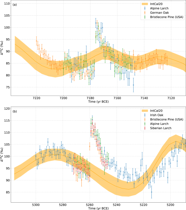
For the 7176 BCE event dendrochronologically dated wood samples from Ireland, supplied by the University of Belfast, and from the Alps, supplied by the University of Innsbruck, were dissected into annually resolved samples weighing 30–60 mg.
For the analyses performed at ETHZ, typically 54 tree-ring samples with four wood blanks (2 BC and 2 KB) and 2 1515 CE reference samples47 each weighing 30–60 mg, were prepared in 15 ml glass test tubes together in a batch (making 60 in total). In a slightly modified procedure following Němec et al.48, samples were first soaked in 5 ml 1 M NaOH overnight at 70 °C in an oven. Then the samples were treated with 1 M HCl and 1 M NaOH for 1 hour each at 70°C in a heat block, before they were bleached at a pH of 2–3 with 0.35 M NaClO 4 at 70 °C for 2 h. The remaining white holo-cellulose was then freeze-dried overnight.
About 2.5 mg dried holo-cellulose was wrapped in cleaned Al capsules49 and converted to graphite using the automated graphitization line AGE50. A measurement set was made up of three oxalic acid one (OX1) and four oxalic acid two (OX2) standards, 27 samples, two cellulose blanks, two chemical blanks, and two 1515 CE reference samples (individual cellulose preparations of the 1515 CE reference is used for at least two measurements) and measured in the MICADAS accelerator mass spectrometer51. Two measurement sets were typically prepared from one set of samples within a week and subsequently measured. A second graphite sample was subsequently prepared and measured from one third of the prepared cellulose samples for quality control purposes.
Two internal wood reference materials from 1515 CE (Pine and Oak) and two different radiocarbon free wood blanks (Kauri Stage 7, KB, and Brown Coal, BC, from Reichwalde) were repetitively analyzed together with the annual samples. While the wood-blanks were used for blank subtraction in the data evaluation process, the 1515 CE references were used for quality control only.
For the analyses performed in Bristol, tree ring samples (20–30 mg) were processed alongside two KB wood blanks and two oak 1524 CE reference samples in 15 ml glass culture tubes. Samples were pretreated following the standard BRAMS wood pretreatment method (code BABAB; following Němec et al.), as described by Knowles et al.52. Around 2.5 mg dried holo-cellulose was combusted, graphitized, and measured using the Bris-MICADAS AMS. Full details of the procedures employed are described by Knowles et al.52.
Several samples were repetitively measured, and a chi-squared analysis showed that the repeated measurements were generally in good agreement with one another. The resulting chi-squared values of the different chronologies are shown in Table 2. Small observed differences are likely due to wood anatomical effects or due to the limitations of cutting tree-rings accurately for species with narrow tree-rings (Supplements S1). The high overall χ2 value events are likely due to regional offset53 and the earlier increase signal in the Bristlecone Pine chronology in the 5259 BCE event.
Table 2 Statistical analysis of the repeated measurements of the different chronologies. Full size table
Modeling
To model the carbon cycle an improved carbon box model based on the model of Güttler et al.54 was used (Supplementary Fig 2). The model of Güttler uses 11 Boxes to simulate the exchange between the global atmosphere biosphere and Oceans. To model the northern and southern hemispheres separately our model was extended to 22 boxes (11 boxes for each hemisphere). The carbon content of each box is distributed according to the respective relative carbon reservoir masses of the corresponding hemisphere. Radiocarbon is produced in the stratosphere and the troposphere of both hemispheres, where 70% is produced in the Stratosphere and 30 % in the Troposphere. The fluxes were adjusted to ensure a correct ∆14C offset between the northern and southern troposphere. Seasonal variability of fluxes was not considered in the model.
The 12C and 14C content of each box after a time step is calculated with
$${N}_{i}^{12}(t+\Delta t)={N}_{i}^{12}(t)+d{N}_{i}^{12}(t)\Delta t$$ (1)
$${N}_{i}^{14}(t+\Delta t)={N}_{i}^{14}(t)+d{N}_{i}^{14}(t)\Delta t$$ (2)
$$d{N}_{i}^{12}(t)=\mathop{\sum}\limits_{j}{F}_{ji}^{12}(t)-\mathop{\sum}\limits_{j}{F}_{ij}^{12}(t)$$ (3)
$$d{N}_{i}^{14}(t)=-\lambda {N}_{i}+\mathop{\sum}\limits_{j}{F}_{ji}^{14}(t)-\mathop{\sum}\limits_{j}{F}_{ij}^{14}(t)+{P}_{i}(t)+{P}_{st,i}$$ (4)
Here \({N}_{i}^{12,14}\) is the \({C}^{12,14}\) content of each box in Gt and λ is the decay constant of 14C. The time step ∆t was chosen to be one month for all the following simulations. The 14C and 12C fluxes are given by the following:
$${F}_{ij}^{12}(t)={F}_{ij,st}\frac{{N}_{i}^{12}(t)}{{N}_{i,st}^{12}},{F}_{ij}^{14}(t)={F}_{ij,st}\frac{{N}_{i}^{12}(t)}{{N}_{i,st}^{12}}\frac{{N}_{i}^{14}(t)}{{N}_{i}^{12}(t)}\frac{{m}_{14}}{{m}_{12}}={F}_{ij,st}\frac{{N}_{i}^{14}(t)}{{N}_{i,st}^{12}}\frac{{m}_{14}}{{m}_{12}}$$ (5)
Here \({F}_{ij,st}\) are the fluxes given in Supplementary Fig. 2. The fluxes are scaled depending on the deviation from the Holocene steady state \({N}_{i,st}^{12}\). The steady state was computed by simulating 200’000 years with the constant production rate \({p}_{st}=1.76\frac{at}{c{m}^{2}s}\). The model does not consider any isotopic fractionation and thus the 14C fluxes scale just as the 12C fluxes.
With this a general expression for all boxes at any time can be achieved.
$$N(t+\Delta t)=N(t)+(\varLambda N(t)+{F}^{T}(t)1-F(t)1+P(t)+{P}_{st})\Delta t$$ (6)
$$F =\left[\begin{array}{cc}{F}^{12}(t) & 0\\ 0 & {F}^{14}(t)\end{array}\right],\varLambda =\left[\begin{array}{cc}0 & 0\\ 0 & -\lambda \end{array}\right],N(t)=\left(\begin{array}{c}{N}^{12}\\ {N}^{14}\end{array}\right),{1}_{i}=1\;{{{\mbox{forall}}}}\;i\\ \,P(t) =Vp(t),{P}_{st}=V{p}_{st}$$ (7)
$${{V}_{i}}=\left\{\begin{array}{cc}0.5\cdot 0.7,\,if\,i=Stratosphere\,N,S\\ 0.5\cdot 0.3,\,if\;i=Troposphere \,N,S \\ 0,\hfill else\hfill\end{array}\right.$$ (8)
The ∆14C of each box for the simulation is calculated by the following expression:
$${\Delta }^{14}{C}_{i}(t)=\frac{\frac{{N}_{i}^{14}(t)}{{N}_{i}^{12}(t)}-\frac{{N}_{TN,st}^{14}}{{N}_{TN,st}^{12}}}{\frac{{N}_{TN,st}^{14}}{{N}_{TN,st}^{12}}}\cdot 1000$$ (9)
Where \({N}_{TN,st}^{12,14}\) are the steady state 12,14C contents of the northern troposphere.
To get a reasonable start state at a given time the production rate for the whole IntCal13 record has been calculated and the simulated state can be loaded at any time before 1950 CE.
The events were evaluated by generating 1000 realizations of the data distributed with the errors of the measurements. For each realization a Gaussian shaped production spike was fitted and the additional production was extracted by integrating the Gaussian production. Since the energy spectrum of the SEPs is softer than the one of the galactic cosmic rays the excess production of the event was mainly produced in the stratosphere (90%) and only 10% in the troposphere. The errors were estimated by using the widths of the resulting distributions.
Geomagnetic field correction
Since the production of 14C in the Earth’s atmosphere is affected by geomagnetic shielding of the flux of SEPs, this effect needs to be accounted for in such a way that all the events are normalized to the same reference standard, specifically to the modern conditions with the dipole moment M = 7.8·1022 A·m2 55. The geomagnetic field has a very complex structure at the Earth’s surface56, but for energetic particles, the dipole moment is the most important since higher momenta decay faster with distance, and the eccentric+tilted dipole approximation is widely used57. Since the true dipole moment is difficult to determine in the past, before the era of direct measurements, an approximation of the virtual axial dipole moment (VADM) is reconstructed from paleo- and archeo-magnetic models58. Accordingly, the geomagnetic-shielding effect on energetic particles is often quantified via the VADM value of M. The modern (epoch 2000) dipole moment is M 0 = 7.8·1022 A·m2. Here we normalize the apparent 14C production Q during different events to the standard modern conditions, viz. the production that would be if the event took place nowadays. For that, we modeled the dependence of Q on M using a broad range of SEP spectra measured during the recent decades59. The spectra are bound between the hardest known spectrum of SEP event on 23-Feb-1956 (GLE 0560) and the softest strong-event spectrum of 04-Aug-1972 (GLE 2460), as shown in Supplementary Fig. 4a. The same plot shows also the global yield function, denoted as Y p (E), of 14C for three VADM values of M = 3, 6 and 9 (x1022 A·m2). The global production function is defined as
$${Y}_{p}(E,M)=\int _{0}^{\pi /2}Y(E)\cdot H(E,M,\theta )\cdot \,\sin (\theta )\cdot d\theta$$ (10)
where Y(E) is the columnar yield function of 14C by protons with energy E in the Earth’s atmosphere61, H(E) is a step-like magnetospheric transmissivity function taking the value of 0 for E < E c and 1 otherwise, where E c is the energy corresponding to the local geomagnetic rigidity cutoff defined by the dipole moment M and the polar angle (co-latitude) θ. The production is higher for a weaker geomagnetic field (smaller values of M) and vice versa. The production of 14C by a specific SEP event with a given proton spectrum J p is defined as the integral of the product of the yield function and the energy spectrum of particles.
$$Q(M)=\int _{0}^{\infty }{Y}_{p}(E,M)\cdot {J}_{p}(E)\cdot dE$$ (11)
The dependence of Q on M is shown in Supplementary Fig. 4b for the two analyzed SEP spectra. In order to compensate for the variable geomagnetic field, we introduce the correction factor, which relates the 14C production at the VADM M to that at the reference field M 0 :
$$C=\frac{Q({M}_{0})}{Q(M)}$$ (12)
The correction factor is shown in Supplementary Fig. 4c for the two SEP spectra. Although the spectra are essentially different (panel a) and the isotope production for the two events is different too (panel b), the correction factor appears robust against the exact spectral shape. This correction factor was further applied to compare the strength of all studied events to the standard conditions, as shown in Table 1.
Reconstructions of the geomagnetic field in the past is a difficult task, and the result can be uncertain. To cover a possible range of VADM values we took a conservative approach and considered two paleomagnetic reconstructions for the last millennia, as shown in Supplementary Fig. 5: a recent GGF100k paleomagnetic model by Panovska et al.40 and a reconstruction by Knudsen et al.41 based on the GEOMAGIA50 database. Although there are many other paleomagnetic reconstructions, these two cover the full range of uncertainties.
The uncertainties of the corrected for the VADM changes 14C production (last two columns in Table 1) are mostly defined by the uncertainties of the actual production (column 3) and VADM uncertainties (columns 4 and 5). The resultant uncertainty of the corrected production was assessed using the Monte–Carlo method by randomly picking pairs of M and Q from the normally distributed values within the ranges shown in Table 1 and computing the mean and the standard deviation of the corrected Q values.