Data
In order to carry out the analysis I use the Fake News Corpus (Szpakowski, 2018), comprised of 9.4 million news items extracted from 194 webpages. Beyond the title and content for each item, the corpus also categorizes each new into one of the following categories: clickbait, conspiracy theories, fake news, hate speech, junk science, factual sources, and rumors. The category for each website is extracted from the OpenSources project (Zimdars, 2017). In particular, the definitions for each category are:
Clickbait
Sources that provide generally credible content, but use exaggerated, misleading, or questionable headlines, social media descriptions, and/or images.
Conspiracy Theory
Sources that are well-known promoters of kooky conspiracy theories.
Fake News
Sources that entirely fabricate information, disseminate deceptive content, or grossly distort actual news reports.
Hate News
Sources that actively promote racism, misogyny, homophobia, and other forms of discrimination.
Junk Science
Sources that promote pseudoscience, metaphysics, naturalistic fallacies, and other scientifically dubious claims.
Reliable
Sources that circulate news and information in a manner consistent with traditional and ethical practices in journalism.
Rumor
Sources that traffic in rumors, gossip, innuendo, and unverified claims.
The labeling of each website was done through crowdsourcing following the instructions as follows (Zimdars, 2017):
Step 1: Domain/Title analysis. Here the crowdsourced participants look for suspicious domains/titles like “com.co”.
Step 2: About Us Analysis. The crowdsourced participants are asked to Google every domain and person named in the About Us section of the website or whether it has a Wikipedia page with citations.
Step 3: Source Analysis. If the article mentions an article or source, participants are asked to directly check the study or any cited primary source. Then, they asked to assess if the article accurately reflects the actual content.
Step 4: Writing Style Analysis. Participants are asked to check if there is a lack of style guide, a frequent use of caps, or any other hyperbolic word choices.
Step 5: Esthetic Analysis. Similar to the previous step, but focusing in the esthetics of the website, including photo-shopped images.
Step 6: Social Media Analysis. Participants are asked to analyze the official social media users associated with each website to check if they are using any of the strategies listed above.
Here, it is important to note that I follow a similar approach as previous studies to classify sources (Broniatowski et al., 2022; Cinelli et al., 2020; Cox et al., 2020; Lazer et al., 2018; Singh et al., 2020). For example, Bovet and Makse (2019) use Media Bias Fact Check to classify tweets according to their crowdsourced classification instead of manually classifying tweet by tweet. This approach has two advantages. First, that it is scalable (Broniatowski et al., 2022) and, secondly, misinformation intent is better captured at the source level than at the article level (Grinberg et al., 2019). Being aware of the potential limitations of this method, the approach offers a benefit: being able to tackle the breadth problem.
Moreover, the fact that I include several misinformation categories is important because most of the existing research has a strong emphasis on distinguishing between fake news and factual news (de Souza et al., 2020; Helmstetter & Paulheim, 2018; Masciari et al., 2020; Zervopoulos et al., 2020). However, not all misinformation is created equal. In general, it is accepted that there are several categories of misinformation delimited by its authenticity and intent. Authenticity is related to the possibility of fact-checking the veracity of the content (Appelman & Sundar, 2016). For example, a statistical fact is easily checkable. However, conspiracy theories are non-factual, meaning we are not able to fact-check their veracity. On the other hand, intent can vary between mislead the audience (fake news or conspiracy theories), attract website traffic (clickbait) or undefined intent (rumors) (Tables 1 and 2).
Table 1 List of sources and their corresponding category. Full size table
Table 2 Comparison with other datasets and papers. Full size table
In the Fake News Corpus, each website is categorized among one of the options and all their articles have the corresponding category. From there, I extracted 30,000 random articles from each category, generating a dataset of 210,000 misinformation articles. For factual news, I used Factiva to download articles from The New York Times, The Wall Street Journal and The Guardian. This resulted in 3177 articles. In total, the database consists of 213,177 articles. I filtered the articles with less than 200 words and those with more than 2000 words, ending up with a database of 147,550 articles. After calculating all the measures (readability scores, perplexity, appeal to morality and sentiment analysis), I deleted all the outliers (lower bound quantile = 0.025 and upper bound quantile = 0.975). This resulted in the final dataset consisting of 92,112 articles with the following distribution by type: clickbait (12,955 articles), conspiracy theories (15,493 articles), fake news (16,158 articles), hate speech (15,353 articles), junk science (16,252 articles), factual news (1743 articles) and rumors (14,158 articles). The 197 websites hosting the 92,112 articles are:
In comparison to other datasets, the one used in this paper includes more sources and more articles than any other:
Computational linguistics
Extant research in the human cognition and behavioral sciences can be leveraged to identify misinformation online through quantitative measures. For example, the information manipulation theory (McCornack et al., 2014) or the four-factor theory (Zuckerman et al., 1981) propose that misinformation is expressed differently in terms of arousal, emotions or writing style. The main intuition is that misinformation creators have a different writing style seeking to maximize reading, sharing and, in general, maximizing virality. This is important because views and engagement in social networks are closely related to virality, and being repeatedly exposed to misinformation increases the likelihood of believing in false claims (Bessi et al., 2015; Mocanu et al., 2015).
Based on the information manipulation theory and the four-factor theory, I propose several parametrizations that can allow to statistically distinguish between factual news and a myriad of misinformation categories. To do so, I calculate a set of quantifiable characteristics that represent the content of a written text and allow us to differentiate it across categories. More specifically, following the definition proposed by (Zhou & Zafarani, 2020) the style-based categorization of content is formulated as a multinominal classification problem. In this type of problem, each text in a set of news articles Ν can be represented as a set of k features denoted by the feature vector \(f \in {\Bbb R}^k\). Through Natural Language Processing, or computational linguistics, I can calculate this set of k features for N texts. In the following subsection I describe these features and their theoretical grounding.
Measuring cognitive effort through grammatical features: readability
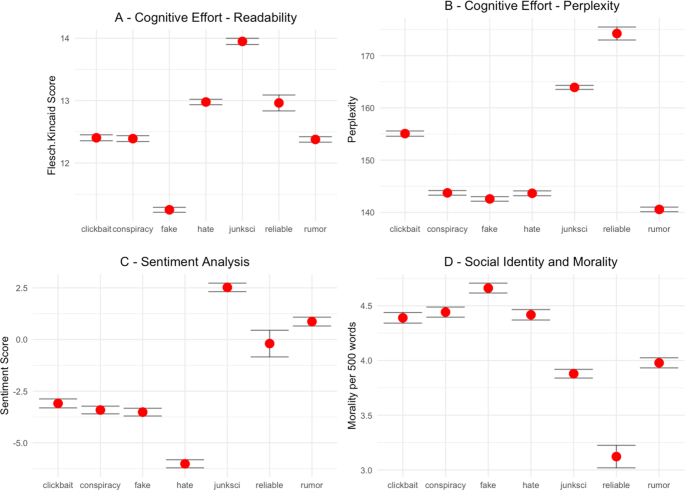
Using sentence length or word syllables as a measure of text complexity has a long tradition in computational linguistics (Afroz et al., 2012; Fuller et al., 2009; Hauch et al., 2015; Monteiro et al., 2018). Simply put, the longer a sentence or word is, the more complex it is to read. Therefore, longer sentences and longer words require more cognitive effort to be effectively processed. The length of sentences and words are precisely the fundamental parameters of the Flesch-Kincaid index, the readability variable.
Flesch-Kincaid is used in different scientific fields like pediatrics (D’Alessandro et al., 2001), climate change (De Bruin & Granger Morgan, 2019), tourism (Liu & Park, 2015) or social media (Rajadesingan et al., 2015). This measure estimates the educational level that is needed to understand a given text. The Flesch-Kincaid readability score is calculated with the following formula (Kincaid et al., 1975):
$${\mathrm{Flesch.Kincaid}}\,{\mathrm{score}}\left( {{\mathrm{FK}}} \right) = 0.39 \ast \left( {\frac{{n_w}}{{n_{st}}}} \right) + 11.8 \ast \frac{{n_{sy}}}{{n_w}} - 15.59$$ (1)
where n w is the number of words, n st is the number of sentences, and n sy is the number of syllables. In this case, n w and n st act as a proxy for syntactic complexity and n sy acts as a proxy for lexical difficulty. All of them are important components of readability (Just & Carpenter, 1980).
While the Flesch-Kincaid score measured the cognitive effort needed to process a text based on grammatical features (the number of words, sentences, and syllables), it does not account for another source of cognitive load: lexical features.
Measuring cognitive effort through lexical features: perplexity
Lexical diversity is defined as a measure of the number of different words used in a text (Beheshti et al., 2020). In general, more advanced and diverse language allows to encode more complex ideas (Ellis & Yuan, 2004), which generates a higher cognitive load (Swabey et al., 2016). One of the most obvious measures for lexical diversity is using the ratio of individual words to the total number of words (known as the type-token ratio or TTR). However, this measure is extremely influenced by the denominator (text length). Therefore, I calculate the uncertainty in predicting each word appearance in every text through perplexity (Griffiths & Steyvers, 2004), a measure that has been used for language identification (Gamallo et al., 2016), to discern between formal and informal tweets (Gonzàlez, 2015), to model children’s early grammatical knowledge (Bannard et al., 2009), measuring the distance between languages (Gamallo et al., 2017) or to assess racial disparities in automated speech recognition (Koenecke et al., 2020).
For any given text, there is a probability p for each word to appear. Lower probabilities indicate more information while higher probabilities indicate less information. For example, the word “aerospace” (low probability) has more information than “the” or “and” (high probability). From here, I can calculate how “surprising” each word x is by using log(p(x)). Therefore, words that are certain to appear have 0 surprise (p = 1) while words that will never appear have infinite surprise (p = 0). Entropy is the average amount of “surprise” per word in each text, therefore serves as a measure of uncertainty (higher lexical diversity) and it is calculated with the following formula:
$$H = - \mathop {\sum }\limits_x p\left( {{x}} \right){\mathrm{log}}_2\,q\left( x \right)$$ (2)
where p(x) and q(x) are the probability of word x appearing in each text. The negative sign ensures that the result is always positive or zero. For example, a text containing the string “bla bla bla bla bla” has an entropy of 0 because p(bla) = 1 (a certainty), while the string “this is an example of higher entropy” has an entropy of 2.807355 (higher uncertainty). Building upon entropy, perplexity measures the amount of “randomness” in a text:
$${\mathrm{Perplexity}}\left( M \right) = \tau ^{ - \mathop {\sum }\limits_x p\left( {{{\mathrm{x}}}} \right)\,{\mathrm{log}}_2\,q\left( x \right)} = 2^H$$ (3)
where τ in our case is 2, and the exponent is the cross-entropy. All else being equal, a smaller vocabulary generally yields lower perplexity, as it is easier to predict the next word in a sequence (Koenecke et al., 2020). The interpretation is as follows: If perplexity equals 5, it means that the next word in a text can be predicted with an accuracy of 1-in-5 (or 20%, on average). Following the previous example, the string “bla bla bla bla bla” has a perplexity of 1 (no surprise because all words are the same and, therefore, predicted with a probability of 1), while the string “this is an example of higher entropy” has a perplexity of 7 (since there are 7 different words that appear 1 time each, yielding a probability of 1-in-7 to appear).
Measuring emotions through polarity: sentiment analysis
The usual way of measuring polarity in written texts is through sentiment analysis. For example, this technique has been used to analyze movie reviews (Bai, 2011), to improve ad relevance (Qiu et al., 2010), to quantify consumers’ ad sharing intentions (Kulkarni et al., 2020), to explore customer satisfaction (Ju et al., 2019) or to predict election outcomes (Tumasjan et al., 2010). Mining opinions in texts is done by seeking content that captures the effective meaning of sentences in terms of sentiment. In this case, I am interested in the determination of the emotional state (positive, negative, or neutral) that the text tries to convey towards the reader. To do so, I employ a dictionary to help in the achievement of this task. More specifically, I employ the AFINN lexicon developed by Finn Årup Nielsen (Nielsen, 2011) one of the most used lexicons for sentiment analysis (Akhtar et al., 2020; Chakraborty et al., 2020; Hee et al., 2018; Ragini et al., 2018). In this dictionary, 2,477 coded words have a score between minus five (negative) to plus five (positive). The algorithm matches words in the lexicon in each text and adds/subtracts points as it effectively finds positive and negative words in the dictionary that appear in the text. If a text has a neutral evocation to emotions will have a value around 0, if a text is evocating positive emotions will have a value higher than 0 and if a text is evocation a negative emotion will have a value below 0. For example, in my sample, one of the highest values in negative emotions (emotion = −32) is the following news from the fake news category reporting about a shooting against two police officers in France: “(…) Her candidacy [referring to Marine Le Pen] has been an uprising against the globalist-orchestrated Islamist invasion of the EU and the associated loss of sovereignty. The EU is responsible for the flood of terrorist and Islamists into France (…)”. In contrast, the following junk science article has one of the highest positive values (emotion = +28): “A new bionic eye lenses currently in development would give humans 3x vision, at any age. (…) Even better is the fact that people who get the lens surgically inserted will never develop cataracts”.
Measuring emotions through social identity: morality
To measure morality, I will use a previously validated dictionary (Graham et al., 2009). This dictionary has been used to measure polarizing topics like gun control, same-sex marriage or climate change (Brady et al., 2017), to study propaganda (Barrón-Cedeño et al., 2019) or to measure responses to terrorism (Sagi & Dehghani, 2014) and social distance (Dehghani et al., 2016). Like in sentiment analysis, morality is measured by counting the frequency of moral words in each text. The dictionary contains 411 words like “abomination”, “demon”, “honor”, “infidelity”, “patriot” or “wicked”. In contrast to previous measures, the technique employed to quantify morality is highly sensitive to text length (with longer texts having higher probabilities of containing “moral” words), therefore, I calculate the morality measure as moral words per 500 words in each text. In addition, since negative news spreads farther (Hansen et al., 2011; Vosoughi et al., 2018), I add an interaction term between morality and negativity by multiplying the morality per 500 words and the negativity per 500 words for each text, this being the main measurement for morality:
$${Morality}_i\left( M \right) = \frac{{{mor}_i}}{{n_{w,i}}} \ast \frac{{{neg}_i}}{{n_{w,i}}}$$ (4)
where mor i is the overall number of moral words in text i, neg i is the absolute number of negative words in text i and n w,i is the total number of words in text i.
Similarities between misinformation and factual news: distance and clustering
For the distance metric I use the Euclidean distance that can be formulated as follows:
$$d_{AB} = \sqrt {\mathop {\sum}
olimits_{i = 1}^n {\left( {e_{Ai} - e_{Bi}} \right)^2} }$$ (5)
Regarding the method to merge the sub-clusters in the dendrogram, I employed the unweighted pair group method with arithmetic mean. Here, the algorithm considers clusters A and B and the formula calculates the average of the distances taken over all pairs of individual elements a ∈ A and b ∈ B. More formally:
$$d_{AB} = \frac{{\mathop {\sum }
olimits_{{{a}} \in {{A}},\,{{b}} \in {{B}}} d\left( {a,b} \right)}}{{\left| A \right| \ast \left| B \right|}}$$ (6)
To add robustness to the results, I also used the k-means algorithm, which calculates the total within-cluster variation as the sum of squared Euclidean distances (Hartiga & Wong, 1979):
$$W\left( {C_k} \right) = \mathop {\sum }\limits_{x_i \in C_k} \left( {x_i - \mu _k} \right)^2$$ (7)
where x i is a data point belonging to the cluster C k , and μ k is the mean value of the points assigned to the cluster C k . With this, the total within-cluster variation is defined as:
$${\mathrm{tot.withiness}} = \mathop {\sum }\limits_{k = 1}^k W\left( {C_k} \right) = \mathop {\sum }\limits_{k = 1}^k \mathop {\sum }\limits_{x_i \in C_k} \left( {x_i - \mu _k} \right)^2$$ (8)
To select the number of clusters, I use the elbow method with the aim to minimize the intra-cluster variation:
$${\mathrm{minimize}}\left( {\mathop {\sum }\limits_{k = 1}^k W\left( {C_k} \right)} \right)$$ (9)
Differentiating misinformation from factual news: multinominal logistic regression
The main objective of this paper is not just to report descriptive differences between reliable news and misinformation sources, but to look for systemic variance among their structural features measured through the four variables. Therefore, it is not enough to report the averages and confidence intervals of each variable for each category, but also analyzing differences and similarities in the light of all variables altogether. This is why I will employ a multinominal logistic regression, a technique suitable for mutually exclusive variables with multiple discrete outcomes.
I employ a multinominal logistic regression model with K classes using a neural network with K outputs and the negative conditional log-likelihood (Venables & Ripley, 2002). This logistic model is generalizable to categorical variables with more than two levels namely {1,…,J}{1,…,J}. Given the predictors \(X_1, \ldots ,X_pX_1, \ldots ,X_p\). In this multinominal logistic regression model, the probability of each level j of Y is calculated with the following formula (García-Portugés, 2021):
$$p_j\left( x \right): = \frac{{{\Bbb P}\left[ {Y = j\left| {X_1} \right. = x_1, \ldots ,X_p = x_p} \right]e^{\beta _{0j} + \beta _{1j}X_1 + \ldots + \beta _{pj}X_p}}}{{1 + \mathop {\sum }
olimits_{l = 1}^{J - 1} e^{\beta _{0l} + \beta _{1l}X_1 + \ldots + \beta _{pl}X_p}}}$$ (10)
for j = 1,…,J − 1 j = 1,…,J − 1 and (for the reference level J = factual news):
$$p_j\left( x \right): = \frac{{{\Bbb P}\left[ {Y = J\left| {X_1} \right. = x_1, \ldots ,X_p = x_p} \right]1}}{{1 + \mathop {\sum }
olimits_{l = 1}^{J - 1} e^{\beta _{0l} + \beta _{1l}X_1 + \ldots + \beta _{pl}X_p}}}$$ (11)
As a generalization of a logistic model, it can be interpreted in similar terms if we take the quotient between (A.1) and (A.2):
$$\frac{{p_j\left( X \right)}}{{p_J\left( X \right)}} = e^{\beta _{0j} + \beta _{1j}X_1 + \ldots + \beta _{pj}X_p}$$ (12)
for j = 1,…,J − 1 j = 1,…,J − 1. If we apply a logarithm to both sides, we obtain:
$${{{\mathrm{log}}}}\left( {\frac{{p_j\left( X \right)}}{{p_J\left( X \right)}}} \right) = \beta _{0j} + \beta _{1j}X_1 + \ldots + \beta _{pj}X_p$$ (13)
Therefore, multinominal logistic regression is a set of J – 1 independent logistic regressions for the probability of Y = j versus the probability of the reference Y = J. In this case, I used factual news as the level of the outcome since I am interested how misinformation differs from this baseline using the following formula:
$${\mathrm{log}}\left( {\frac{{P\left( {{\mathrm{cat}} = j = {\mathrm{fake}}} \right.}}{{P\left( {{\mathrm{cat}} = J = {\mathrm{reliable}}} \right)}}} \right) = \beta _{0j} + \beta _{1j}\left( r \right) + \beta _{1j}\left( p \right) + \beta _{1j}\left( s \right) + \beta _{1j}\left( m \right)$$ (14)
where s = sentiment, m = morality, r = readability and p = perplexity. This method will allow us, beyond the fingerprints of misinformation described before, to quantify the differences between factual news and non-factual content.