Biological data
The CPR Survey is a long-term, sub-surface marine plankton monitoring programme consisting of a network of CPR transects towed monthly across the major geographical regions of the North Atlantic. It has been operating in the North Sea since 1931 with some standard routes existing with a virtually unbroken monthly coverage back to 194621,22. The CPR survey is recognised as the longest sustained and geographically most extensive marine biological survey in the world23. The dataset comprises a uniquely large record of marine biodiversity covering ~1000 taxa over multidecadal periods. The survey determines the abundance and distribution of phytoplankton and zooplankton (including fish larvae) in our oceans and shelf seas. Using ships of opportunity from ~30 different shipping companies, it obtains samples at monthly intervals on ~50 trans-ocean routes. In this way the survey autonomously collects biological and physical data from ships covering ~20,000 km of the ocean per month, ranging from the Arctic to the Southern Ocean24.
The CPR is a high-speed plankton recorder that is towed behind ‘ships of opportunity’ through the surface layer of the ocean (~10 m depth)9. Water passes through the recorder and plankton are filtered by a slow-moving silk (mesh size 270 µm). A second layer of silk covers the first and both are reeled into a tank containing 4% formaldehyde. Upon returning to the laboratory, the silk is unwound and cut into sections corresponding to ten nautical miles and ~3 m3 of filtered sea water25. There are four separate stages of analysis carried out on each CPR sample, with each focusing on a different aspect of the plankton: (1) overall chlorophyll (the phytoplankton colour index; PCI); (2) larger phytoplankton cells (phytoplankton) in the case of this study we have just analysed diatoms which are all on the large size compared with smaller flagellates and coccolithophores that are also recorded.; (3) smaller zooplankton (zooplankton ‘traverse’); and (4) larger zooplankton (zooplankton ‘eyecount’). The collection and analysis of CPR samples have been carried out using a consistent methodological approach, coupled with strict protocols and Quality Assurance procedures since 1958, making the CPR survey the longest continuous dataset of its kind in the world24. Of the more than 200 phytoplankton species recorded by the Survey we analysed a sub-set of data consisting of over 49 diatom species/taxonomic entities (Supplementary Table 1). The selection of taxa was based on their frequency of occurrence, consistency of recorded taxa across the whole time-series (1958–2017). Rare species were removed during the selection to make the dataset statistically more robust. Practically, we chose diatoms that had an annual abundance >0 for at least 50 years.
Potential biases and limitations
The CPR survey currently records ~1000 plankton entities (many to species level) in routine taxonomic analysis with strict Quality Assurance protocols in operation for its sampling and plankton counting procedures since 1958. Due to the mesh size of CPR silks, many plankton species are only semi-quantitatively sampled owing to the small size of the organisms. In the case of phytoplankton there is thus a bias towards recording larger armoured flagellates and chain-forming diatoms and that smaller species abundance estimates from cell counts will probably be underestimated in relation to other water sampling methods24. However, the proportion of the population that is retained by the CPR silk reflects the major changes in abundance, distribution and specific composition, i.e. the percentage retention is roughly constant within each species even with very small-celled species down to 10 µm19,24. In certain circumstances clogging due to increased loading associated with mucilage and high densities of plankton may contribute to the number of small plankton captured. Despite these sporadic occurrences the CPR has still been shown to capture a consistent fraction of the in situ abundance of the species assayed25. A similar potential under estimation of zooplankton abundances has recently been thoroughly statistically explored and found that while the CPR survey does underestimate abundance in some cases it provides a realistic quantification of both temporal (i.e. seasonal and diel scales) and spatial (i.e. regional to basin-scale) changes in zooplankton taxa (In this case for the species Calanus finmarchicus)24,26. The study also showed that while the CPR sampling is restricted to surface waters ~10 m in depth the seasonal and diel patterns of abundance of C. finmarchicus were positively correlated to patterns of abundance to a depth of 100 m26.
While all sampling and analytical tools for measuring plankton have their own individual strengths and weaknesses, the CPR Survey has had perhaps the most well documented and transparent examination of its consistency and compatibility of any ecological time series over time21,23. Perhaps the most obvious limitation of CPR sampling is its underestimation of components of the plankton, e.g. large plankton like fish larvae and delicate gelatinous plankton. This has been well documented and users of the data are advised of the CPR’s potential biases24,25. It is also widely recognised that all plankton sampling systems have their own limitations and nuances and all underestimate abundance to some degree and that the varying mechanisms are not always directly comparable24,27. A detailed study has been conducted on flow rate and ship speed on CPR sampling28 given that the speed of the ships has, in some circumstances, increased since the 1960s, which may impact sample efficiencies. However, no significant correlation was found between the long-term changes in the speed of the ships and two commonly used indicators of plankton variability: Phytoplankton Colour and Total Copepods indices24. This absence of relationship may indicate that the effect found is small in comparison with the influence of hydroclimatic forcing24,28. For further details on the technical background, methods, consistency, and comparability of CPR sampling, see ref. 21.
Hydroclimatic indices
The North Atlantic experiences climate variability on multidecadal scales often referred to as AMV29. The AMV has been operating over the last few centuries as an observed phenomenon and has also been identified at millennial timescales using paleoclimatic proxy data and models. However, identifying the mechanisms behind the AMV, be they externally forced or driven by internal dynamics or a combination of both is still widely debated29,30,31. Here we use the AMO index to reflect this low frequency variability in the North Atlantic. The AMO is a large-scale oceanic phenomenon and a source of a natural variability in the range of 0.4 °C in the oceanic regions of the North Atlantic32. The AMO is also detected in paleoclimatic reconstructions with a cycle ranging from 60 to 100 years33. The index is calculated from the Kaplan SST dataset which is updated monthly and represents an index of the North Atlantic temperatures; we used the unsmoothed version of the index (http://www.esrl.noaa.gov/psd/data/timeseries/AMO/). The AMO has been related to various biological shifts in the North Atlantic sector34.
NAO index is a basin scale alternation of atmospheric mass over the North Atlantic between the high pressures centred on the subtropical Atlantic and low pressures around Iceland and is a prominent mode of variability with important impacts from the polar to subtropical Atlantic and surrounding landmasses. The index is calculated on the surface sea-level pressure difference between the Subtropical (Azores) High and the Subpolar Low (https://www.ncdc.noaa.gov/teleconnections/nao/).
We also used Northern Hemisphere temperature anomalies (HadCRUT4). This climatic index was developed by the Climatic Research Unit (University of East Anglia) and the Hadley Centre (UK Met Office)35. CRUTEM4 and HadSST3 are the land and ocean components of this dataset, respectively (https://crudata.uea.ac.uk/cru/data/temperature/). Global temperature anomalies have been frequently correlated with long-term changes in biological and ecological systems36.
Climatic data (wind and sea surface temperature)
We used wind intensity (W wind), the zonal (U wind, from west to east) and meridional (V wind, from south to north) components of the wind to investigate potential relationships between wind intensity and direction and diatom abundance. Wind intensity and direction influence the structure of the water column and are known to be important environmental parameters for diatoms37. Wind intensity and direction (monthly basis and spatial resolution of 2.5° latitude × 2.5° latitude) was obtained from the National Centers for Environmental Prediction and the National Center for Atmospheric Research, who have run a reanalysis project using a state-of-the-art analysis/forecast system to perform data assimilation using past data from 1948 to the present38. For the analysis we constructed a spatially gridded (2.5° latitude × 2.5° longitude) dataset for the northeast Atlantic region (40.5°N to 65.5°N and 30.5°W to 10.5°E) and the North Sea (52°N to 60°N and 2°W to 10°E), corresponding to the period 1958–2017.
SST was extracted from the Extended Reconstructed Sea Surface Temperature (ERSST)_V5 data-set, which is derived from a reanalysis of the most recently available International Comprehensive Ocean-Atmosphere Data Set SST data. Improved statistical methods were used to produce a stable monthly reconstruction from relatively sparse data39. For this analysis we constructed a spatially gridded (2° latitude × 2° longitude) annual average SST dataset for the Northern Hemisphere.
Spatialised standardised principal component analysis on total diatoms in the northeast Atlantic
We calculated the sum of the abundance of all diatoms recorded semi-quantitatively by the CPR survey (264,837 samples). Because data from the CPR survey are not regularly spaced in time and space, we interpolated the data for total diatoms on a 2-monthly basis between 1958 and 2017 using an inverse squared distance method with a search radius of 150 km and a number of values for calculating the weighted mean ranging between 3 and 2040,41. The boundary of the studied region ranged from 40.5°N to 65.5°N and from 30.5°W to 9.5°E for every 1° latitude × 1° longitude; inside the area, we kept geographical cells that had at least 50 non-zero estimates of total diatom abundance. Annual means were subsequently calculated for every geographical cell. We kept cells that had at least 30 years of estimates of total diatom abundance.
A spatialised standardised PCA was performed on the matrix 1066 geographical cells (26 latitudes × 41 longitudes) × 60 years. The matrix of standardised eigenvectors 1066 × 1066 geographical cells represented the linear correlations with the principal components that had a dimension of 60 years41. We applied a broken-stick model to test the significance of the different axes of the PCA using 10,000 simulations42.
Standardised principal component analysis on species of diatoms in the North Sea
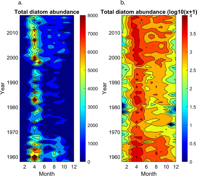
We calculated the abundance of all diatom species (including total diatom abundance) occurring in the North Sea (52°N to 60°N and 2°W to 10°E) on a monthly basis for the period 1958–2017. Long-term monthly changes in total diatoms were examined first in relation to the hydro-climatic indices (AMO, NAO and NHT). Data were then annually averaged and a standardised PCA was performed on the matrix 60 years × 49 species/taxa. This analysis therefore focussed on all species or taxa of diatoms, which was not investigated on the first PCA that jointly considers spatial and temporal changes in total diatom abundance. Here also, we applied a broken-stick model to test the significance of the different axes of the PCA using 10,000 simulations42.
Relationships between changes occurring in the northeast Atlantic and the North Sea
We correlated the long-term changes in the first principal components (PCs) originating from the PCA performed at the scale of the North Atlantic with changes in diatom abundance at the species or taxonomic level. For this analysis, we represented changes in diatom species in addition to a PC when the PC-species correlation was higher than 0.7 (i.e. percentage of explanation >49%).
Maps of correlations
We calculated maps of correlation between W, U, V wind and SST and the first PC originating from the PCA performed on total diatoms at the northeast Atlantic scale. For this analysis, we applied an order-2 simple moving average to alleviate the influence of short-term higher frequency variability. This analysis was conducted for the time period 1958–2017.
Correlation analyses between variables