Data
To study jet stream states over Eurasia we used ERA5 reanalysis data60 for the zonal-mean zonal wind (u) over the area 25°−80°N, focusing on the Eurasian sector (25°W–180°E), for the pressure levels 800hPa-100hPa, and for the months July and August. The size of the domain and the pressure levels were tested and the results were found to be insensitive to changes (e.g. 0–90°N, or pressure levels 1000hPa-100hPa). The data are in a 0.28° × 0.28° spatial resolution and daily values were calculated from 6-hourly data (in particular from the timesteps 00:00, 06:00, 12:00 and 18:00). Other variables used and presented in composite maps, such as mean and maximum surface temperature (used to calculate the heatwave metrics, see “Heatwave definition, metrics, and trends”) and zonal (u) and meridional (v) wind at the 250hPa pressure level were also retrieved from the ERA5 datasets.
Heatwave definition, metrics, and trends
Although there is no universal definition for heatwaves, there are some criteria and thresholds that have been used and tested extensively in the literature. Main characteristics of a heatwave are the physical one which describes its intensity, referring to the temperature ranges reached, the temporal that refers to its duration, and the spatial, which describes the spatial extent of a heatwave. Here we define a heatwave day based on the following criteria:
Temperature threshold: the daily maximum temperature has to exceed the 90th percentile of the maximum temperature distribution of the period studied based on a centered 15-day window (Tmax >90th percentile), following Fischer and Schär 61 .
Temporal extension: we define heatwaves as at least 3 62 or 6 61 consecutive days of temperature threshold exceedance. In the main manuscript we present the results referring to long heatwaves (≥6 consecutive days), while results for shorter heatwaves (≥3 consecutive days) are presented in the SI.
Spatial extent: we define an event as a heatwave if it exceeds an area of 40.000 km2 within a 4° × 4° sliding window (similar to Stefanon et al.63). Different sliding windows were tested and did not have a significant effect on the heatwave detection.
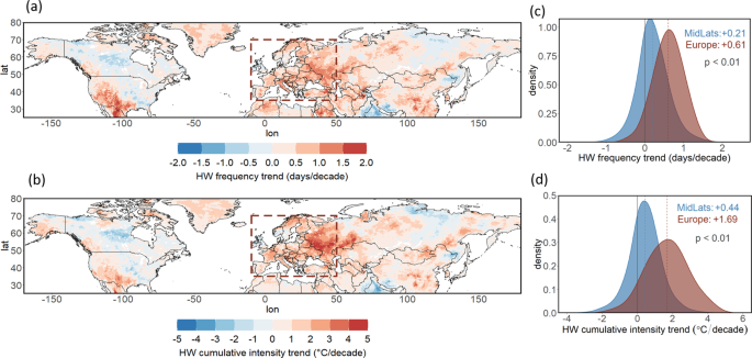
Apart from the heatwave frequency we are also interested in the heatwave intensity. Here we look at the heatwave cumulative intensity, as defined by with Perkins-Kirkpatrick and Lewis3, which refers to the integration of heat exceedance over the threshold for each heatwave event. When referring to a whole region, we additionally aggregate the heat exceedance for the whole spatial extent:
$${heatwave}\,{cumulative}\,{intensity}={\sum }_{1}^{{gp}}\;{\sum }_{1}^{d}(T{\max }-{T{\max }}_{90{th}})$$ (1)
where gp is the number of land grid points for each region, d is the number of consecutive heatwave days, Tmax the maximum daily temperature and Tmax 90th the 90th percentile of the maximum temperature distribution of the whole time period 1979–2020.
The heatwave cumulative intensity is a useful metric as it integrates in a single number all the characteristics of a heatwave: intensity, duration and spatial extent. This way it enables easier comparisons between different regions or years. Additionally, considering the excess heat experienced once the heatwave threshold is exceeded makes this metric more impact-relevant3.
In all cases where heatwave cumulative intensity is aggregated for a certain region, only the land grid points are considered and the data are weighted by the cosine of the latitude to account for the different size of the grid cells between different latitudinal zones.
All trends reported in this study, such as the trends of the heatwave metrics and those of the double jet frequency and occurrence, are simple linear trends calculated as the slope of the least squares line of each variable against time. Additionally, a LOESS regression smoothing has been applied in the case of the trends of the SOM similarity indices in Fig. 3d, e. For the comparison of distributions, the Kolmogorov-Smirnov test was used.
Identification of jet stream states
In order to detect double jet configurations in the vertical zonal-mean zonal wind field, we used a neural network-based, unsupervised clustering algorithm, Self-Organizing Maps (SOM35,64). SOMs have been used a lot in recent decades in atmospheric sciences31,65 and they provide a flexible alternative to other clustering algorithms, such as k-means and hierarchical clustering. The SOM algorithm starts with randomly initialized weight vectors (c), followed by a sampling step, during which a random input vector (x) is compared to all weight vectors until its Best Matching Unit (BMU) is detected according to a distance metric (here we use sum of squares). Next, the BMU and its neighboring units are updated to become more similar to the newly added input vector, according to the following function:
$${{{{{{\bf{c}}}}}}}_{{{{{{\bf{k}}}}}}}\left(t+1\right)={{{{{{\bf{c}}}}}}}_{{{{{{\bf{k}}}}}}}\left(t\right)+\alpha \left(t\right)\times {h}_{{ck}}(t)\times [x\left(t\right)-{{{{{{\bf{c}}}}}}}_{{{{{{\bf{k}}}}}}}\left(t\right)]$$ (2)
where c k the BMU weight vector, α the learning rate parameter that decreases with each iteration t, and h ck a neighborhood function determining how many neighbor nodes surrounding the BMU will be affected. Here, the bubble type neighborhood function was used:
$${h}_{{ck}}(t)=F(\sigma (t)-{d}_{{ck}})$$ (3)
where σ is the neighborhood radius that decreases linearly with iteration (t) until it reaches 0, when no neighbor nodes are updated anymore, d ck the Euclidean distance between the BMU (c) and another one of the SOM nodes (k), and F(x) is a step function that takes the value 1 as long as the neighborhood radius remains larger than the Euclidean distance, and the value 0 when the radius becomes equal to it.
This procedure is repeated for each one of the input vectors (the algorithm goes back to the sampling step) until the final SOM array does not change anymore. The SOM finalization is achieved when all input vectors have been assigned to their BMU. The neighborhood function included in the SOM algorithm is the element that makes this method different from other clustering techniques, such as k-means, as it allows for a topological ordering of the SOM clusters in the final SOM array, which represents the structure of the input data.
One of the choices that has to be made a priori with SOMs is how many clusters will be employed and this heavily depends on the scope of the study and the application and the degree of generalization that one wants to achieve. For our analysis, we tried different SOM sizes (from 2 to 6, not shown) and found that 3 SOMs represent the different jet stream states that we are interested in to a good degree. More than 3 SOMs produced very similar clusters, while 2 SOMs resulted in too general patterns. Additionally, we tested k-means and hierarchical clustering on the same data and with the same number of clusters (2–6) and the results were fairly similar (not shown).
Furthermore, due to the inherent stochasticity of the SOM algorithm, slightly different results may be obtained from different random initializations and therefore multiple random runs are recommended66. Here we use 10 random runs and choose the SOM array that better represents the input data according to the quantization error that measures the goodness of the final SOM in terms of similarity of the SOM clusters to the contained data vectors67:
$${quantization}\,{error}=\frac{1}{N}\sum {{{{{\rm{||}}}}}}{\vec{{{{{{\bf{x}}}}}}}}_{{{{{{\bf{i}}}}}}}-{{{{{{\bf{c}}}}}}}_{{\vec{{{{{{\bf{x}}}}}}}}_{{{{{{\bf{i}}}}}}}}{{{{{\rm{||}}}}}}$$ (4)
where N is the number of data vectors x and c its best matching unit, i.e. the weight vector of the SOM cluster in which it is classified.
Apart from testing different numbers of SOM clusters and running 10 random initializations, we performed sensitivity analysis regarding the months used as input for the SOMs, and the spatial domain. Initially, June-July-August (JJA) data were tested, but the results showed that June has a fairly different behavior compared to July and August in terms of the jet stream, being more of a transitional month between spring and summer. This might be related to the fact that the most pronounced thermal gradient over the Arctic circle is seen in high-summer months, due to the largest differences in land versus sea warming25. To test whether the results are robust for an extended warm period, we projected the three SOMs defined in July and August on May, June, and September (Fig. S4). Figure S5 shows the distribution of the three jet stream states among the different months of this extended period. May and June, primarily, and September to a lesser degree, are dominated by the mixed jet stream state. On the other hand, double jets are almost exclusively a July and August feature, as they hardly occur in the other months. Nevertheless, even when taking into account May-September (MJJAS), the composites of mean temperature and heatwave cumulative intensity (Fig. S4j-l and m-o) remain consistent with the ones seen in Fig. 2 for July-August only. Additionally, the significant upward trends in frequency and persistence of double jets (Fig. S4d-f) are also detected in the MJJAS analysis.In addition, although a lengthening of the mean European summer period has been observed68,69 and often early summer heatwaves may have greater impacts on mortality70, most of the severe European heatwaves are taking place in high-summer(July-August)9. For these reasons we decided to focus this analysis on July-August (JA) only, similarly to previous studies71.
For the spatial domain, we tested both the whole hemisphere and the Eurasian sector only. The results were consistent (not shown), with double jets always showing up in one of the clusters with a similar frequency of occurrence, and therefore we chose to continue the analysis using the jet states over the Eurasian sector, as they are more relevant for heat extremes over Europe.
Therefore, SOMs were applied on the vertical zonal-mean zonal wind values of different pressure levels (from 800hPa up to 100hPa, at levels taken every 100hPa) of the daily ERA5 data of July and August for the period 1979–2020. Before applying the clustering algorithm, the zonal wind fields were weighted by the cosine of the latitude to account for the different size of the grid boxes. The three jet stream states obtained by the SOMs are characterized by the composites of the days belonging to each of them, by a total frequency of occurrence for the whole period, and by their annual frequency and persistence. The annual frequency refers to the number of days that were clustered to each of those jet stream states (SOMs) per year and the annual persistence refers to the maximum number of consecutive days clustered to each of them per year.
Next, focusing on the most persistent double jet events, and in particular those with persistence exceeding the 90th percentile, we further clustered the meridional wind at 250hPa (v250) over Eurasia of those events in order to analyze dominant wave patterns. We clustered v250 in two SOMs and applied 10 random runs, choosing the one with the smallest quantization error. In order to check for the existence of trends in the occurrence of the two v250 clusters, we calculated a similarity index among the two v250 composites and the daily fields of v250. Then, the linear trend of those indices were estimated, and additionally, to account for non-linear trends a smoothed LOESS regression curve was applied (using a span of 0.75).All SOM implementations were done in R with the use of the latest version of the “kohonen” package72.
Links of jet stream states and climate
Composites of different variables were made for the days belonging to each one of the three jet states described above. The composites of the zonal wind at the 250hPa level (u250) and of mean surface temperature were calculated for detrended and deseasonalized data and are presented in terms of anomalies from climatology, which was taken as the mean state of all days of the study period (July and August for 1979–2020). For the composites of heatwave cumulative intensity, we detrended the data by removing from each grid point the land mean trend of the Northern Hemisphere midlatitudes (25–70°N). The composites are then presented in terms of relative anomalies (%) compared to climatology.
In order to assess the links between jet stream states and heatwave metrics, we determined linear regression models to quantify the part of the observed heatwave variability explained by the jet stream in a linear model. To account for biases due to potential trends, we first detrended the regressors (jet state frequency and persistence) and the heatwave metrics (frequency and cumulative intensity).
Further, we calculated the estimated trends in the heatwave metrics at each grid point based on the linear regression model of the previous step. We used the regression parameters for the models calculated for the detrended data to estimate the heatwave trends using the non-detrended regressor (jet frequency and persistence). This way we can compare the estimated trend to the observed one. For the observed trend, we use the residual trend for each grid point after having subtracted the mean midlatitude-land trend. As a first-order approximation, we assume that the thermodynamical contribution to the increase in heatwaves is approximately similar for different midlatitude regions. The observed residual trend is the one that we can then attribute to other changes, such as dynamical changes in the jet stream and local feedbacks.