Data acquisition and processing
Cruise NBP19-02 took place between January and March 2019 on the United States Antarctic Program icebreaking vessel RV Nathaniel B. Palmer as part of the wider National Science Foundation–Natural Environment Research Council funded International Thwaites Glacier Collaboration involving UK, US and multi-national affiliates. Onboard, we collected underway multibeam swath bathymetry, sub-bottom profiler data and recovered marine sediment cores to improve our understanding of Thwaites Glacier history. For this paper, we focus on datasets collected by the deployment of a 6,000-m-depth-rated free-swimming Kongsberg HUGIN AUV. The AUV, operated by the Swedish Research Council and maintained by the University of Gothenburg, was trialled and underwent first deployments in polar waters during the cruise. ‘Ran’ is equipped with a variety of oceanographic sensors, as well as a full suite of geophysical instrumentation. Here we show data collected using an AUV-mounted single-head Kongsberg EM2040 multibeam echo-sounder and a dual-frequency Edgetech 2205 sidescan sonar. Both sonars enabled the collection of high-resolution images of the sea bed at a resolution unrivalled for shelf regions around the West Antarctic Ice Sheet.
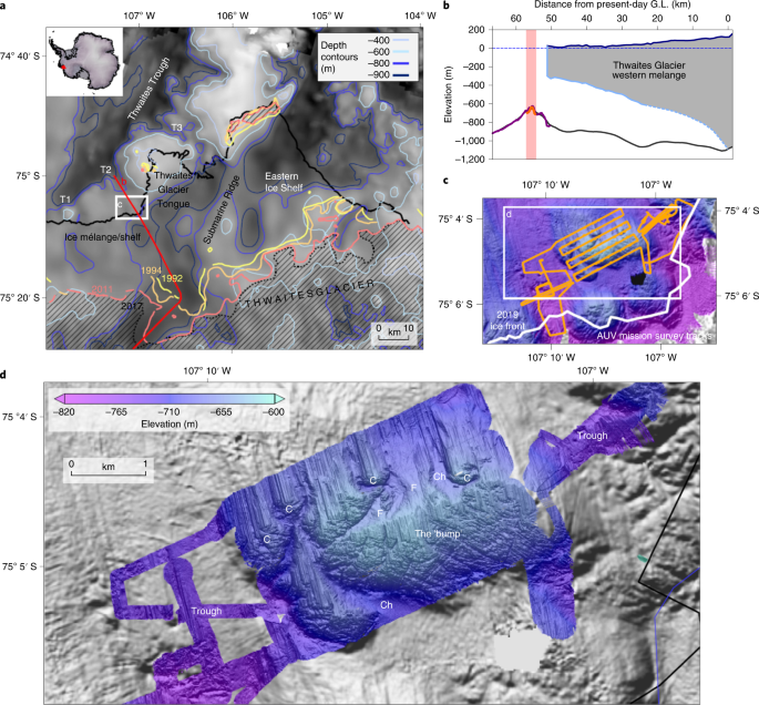
AUV mission 009 deployed the HUGIN at 75° 04.21′ S, 106° 58.89′ W, at 22:07h on 28 February 2019. Recovery occurred at 15:33h on 1 March 2019 at 75° 05.409′ S, 107° 10.925′ W. The total mission time was 17 h 26 min. Navigation was achieved by coupling an onboard INS (inertial navigation system consisting of accelerometers and gyros) with two 12 kHz Universal Transponder Positioning (UTP; cNODES) units deployed at known locations that served as call and response range-positioning for the vehicle. In addition, the vehicle operated using a Doppler velocity log whereby it tracked the sea floor or sea surface via dead reckoning. Acquisition heights varied during the survey between 50 m and 95 m. Processing of navigation data was undertaken onboard in Kongsberg proprietary NavLab software. However, owing to noise from the first UTP station, the filtered navigation required further processing subsequent to the cruise by Kongsberg engineers in Norway.
Processing of the AUV multibeam swath bathymetry data using a first-pass cleaned navigation was undertaken in MB system while onboard the Palmer. The steps involved (1) extraction of navigational and attitude data, (2) bathymetry data conversion, (3) ping editing to remove spurious soundings and (4) gridding. Because of the varied flying height, an onboard gridded dataset was produced at a conservative 1.5 m grid cell size, which formed the basis of most bathymetric analysis in this paper. We gridded using a Gaussian-weighted mean algorithm in the mbgrid program, adopting a spline interpolation to fill grid cells not filled by swath data for gaps up to six grid cells in size. The grid was exported in an ESRI ASCII format for manipulation in a geographic information system. The 1.5 m grid was used for the majority of observations made in our analyses.
Post-processing of the AUV data by Kongsberg technicians removed noise problems associated with the first of the two UTPs that hampered processing of the vehicle’s navigation onboard. In post-processing, we removed fixes from the first UTP entirely. Consequently, for the start of the mission, the AUV ran on dead reckoning with GPS fix until the second UTP was encountered after which navigation was determined by UTP-INS. A cleaned and filtered real-time navigation using a best-fit solution was output via NavLab. Loops (avoidance turns) in the vehicle track, of which there were several, were removed, and a static shift of 95 m at 130° was applied. A second grid with improved resolution of 0.7 m was produced for subsequent visualization and verification of our analyses from the coarser, 1.5 m gridded dataset.
Images of the sea floor acquired by the AUV’s sidescan sonar were replayed and exported using Kongsberg reflection post-acquisition visualization software, isolating the high-frequency channel (400 kHz). Each image was slant-range corrected and processed with a pixel size of 0.05 × 0.05 m.
Geomorphological mapping of landforms
Glacial landforms were mapped from the gridded multibeam datasets in a geographic information system using associated hillshade surfaces and corresponding sidescan sonar imagery for guidance. All mapping was undertaken at horizontal scales between 1:500 and 1:5,000. We used the original 1.5 m multibeam grid for the majority of feature mapping but updated the map with subsequent mapping work in selected areas using digitized landforms from the later post-processed 70 cm grid. Any updates to the map at this second stage were geo-located to be consistent with the original mapping using an XY shift. As the landform map was generated before secondary post-processing of the AUV data, it should be noted that the completed map has a small XY offset of approximately 95 m at 130°. However, the data as a whole are internally consistent, meaning the interpretations and subsequent geometric analysis of the ribs are not subject to any appreciable change. Landforms were classified by geometry, independent of their genetic interpretation following best practices described in a variety of glacial geomorphological literature. Extended descriptions of the landforms and their genetic classification are included in Supplementary Section A2.
To extract landform statistics from the bathymetric data, we employed a semi-automated picking approach. Profiles were extracted from the bathymetry along the sets of ribs of interest, sampled at a horizontal resolution of 10 cm. The extracted long profiles were detrended and mean-adjusted by removing a least-squares regression from the profile. Subsequently, the data were filtered by subtracting a 100-point adjacent averaging smooth of the detrended data, which served to remove long-wavelength features in the bathymetry profile while retaining the finer details and geometry of smaller-scale landforms of interest. From the filtered and detrended data, a manual baseline was digitized that assigned nodes to the troughs between ribs and interpolated between them. We subtracted the baseline from the data so that the ribs in series were levelled to a zero horizon. A peak analysis tool was then used to identify rib crests in the processed profiles from which height from baseline (amplitude) and peak-to-peak spacing were automatically derived.
Tidal model
To investigate the potential role of tides in forming sea-floor landforms, we extracted predicted tidal amplitudes from a tidal model of the global ocean for a location seaward of the Thwaites Glacier front (108° W, 74° S). This was carried out to provide a handle on the expected modern-day tidal amplitudes at the ice-shelf margin and to establish the dominant tidal constituents driving ice-shelf and grounding-line flexure on both short and long timescales. We used the Oregon State University TPXO-9 Global Tidal Model for analysis28. The model includes complex amplitudes of relative sea-surface elevations for eight primary (M2, S2, N2, K2, K1, O1, P1 and Q1), two long-period (Mf and Mm) and five non-linear (M4, MS4, MN4, 2N2 and S1) harmonic constituents.
The time window chosen for comparison covered the period 22 March 2020 to 4 September 2020 and was sampled at hourly intervals encompassing nearly 12 spring–neap cycles (166 days on plotted axis in Fig. 4). The dates selected for the tidal record comparison began at the end of the austral summer, and were forecast through to the end of the following austral spring. The late March start date for the time series reflects an attempt to correlate the landform record with a time period in which West Antarctica is generally at its warmest, and sea ice is at a minimum in the Amundsen Sea. Although investigations of the seasonal variability in the properties of CDW in the easternmost Amundsen Sea embayment generally indicate a thicker and slightly warmer deep water layer during winter38, we view the end of summer as the most likely time interval in which rapid ice sheet retreat events might be triggered. Modelling studies indicate that the largest southward transport of heat and the thickest CDW layer peaks in the March–May period. For guiding our choice, other rapid changes in Antarctic glaciers have typically been observed to have initiated in the late summer period: for example, the Larsen A Ice Shelf disintegrated in January 1995, while Larsen B collapsed during the period 31 January to March 2002, and Wilkins Ice Shelf underwent partial collapse through February and March of 2008. Whereas collapses of the Antarctic Peninsula ice shelves have mainly been triggered by surface melting and hydrofracture as a result of atmospheric warmth, changes at Thwaites Glacier are likely to be ocean or sea-level instigated. Although there is no explicit link between the timing of major calving events and grounding-zone retreat, we note observations of major changes in Thwaites Glacier in March of previous years: Thwaites had a partial outburst of its western mélange in the period immediately following our AUV survey in early March 2019, while the large iceberg B-22 previously calved from the Thwaites Ice Tongue in mid-March 2002.
Analysis of rib landforms
The periodograms in Fig. 4 of the main manuscript investigate the dominant periods (frequencies) in the series of ribs compared with the frequency content of the tidal series. The dominant frequencies describe important periodicities in the data. The periodograms were produced using a fast Fourier transform implemented in OriginLab. Frequency corresponds to cycles per unit of time. In this case, the unit of time was set to 1 calendar day so that periods equate to 1/peak frequency. For the tidal model, we filtered the hourly modelled tidal amplitude outputs from the TPXO-9 model using a 24-point percentile filter with a percentile value set at 99 (Supplementary Fig. 13). This corresponded to replacing the signal point with the 99th percentile value of the data points in the moving data window. The resultant filtered dataset removes the 24, 12 and 6 h tidal periodicities that dominate the full-resolution tidal dataset (Supplementary Fig. 13b), preserving and tracking closely the daily peak tidal height. We compared this approach with a method that decimated the data to a single time per day. Both achieve similar results in emphasizing the dominance of a fortnightly spring–neap cyclicity in the daily tidal values.
For the ribs, we analysed the dominant frequencies in the amplitude data as a series. Since the amplitude data are already detrended and extracted from the initial topography, they represent an appropriate way of investigating periods in the data. However, periodograms of the filtered and mean-adjusted topography produce results with no discernible differences. In each FFT (Fast Fourier Transform) analysis, we carried out the routine using a Hanning window and display the amplitude as a function of frequency.